blog
An Overview of Various Auxiliary Plan Nodes in PostgreSQL

All modern database system supports a Query Optimizer module to automatically identify the most efficient strategy for executing the SQL queries. The efficient strategy is called “Plan” and it is measured in terms of cost which is directly proportional to “Query Execution/Response Time”. The plan is represented in the form of a tree output from the Query Optimizer. The plan tree nodes can be majorly divided into the following 3 categories:
- Scan Nodes: As explained in my previous blog “An Overview of the Various Scan Methods in PostgreSQL”, it indicates the way a base table data needs to be fetched.
- Join Nodes: As explained in my previous blog “An Overview of the JOIN Methods in PostgreSQL”, it indicates how two tables need to be joined together to get the result of two tables.
- Materialization Nodes: Also called as Auxiliary nodes. The previous two kinds of nodes were related to how to fetch data from a base table and how to join data retrieved from two tables. The nodes in this category are applied on top of data retrieved in order to further analyze or prepare report, etc e.g. Sorting the data, aggregate of data, etc.
Consider a simple query example such as…
SELECT * FROM TBL1, TBL2 where TBL1.ID > TBL2.ID order by TBL.ID;Suppose a plan generated corresponding to the query as below:
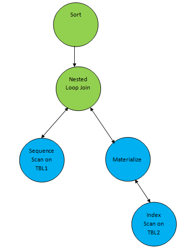
So here one auxiliary node “Sort” is added on top of the result of join to sort the data in the required order.
Some of the auxiliary nodes generated by the PostgreSQL query optimizer are as below:
- Sort
- Aggregate
- Group By Aggregate
- Limit
- Unique
- LockRows
- SetOp
Let’s understand each one of these nodes.
Sort
As the name suggests, this node is added as part of a plan tree whenever there is a need for sorted data. Sorted data can be required explicitly or implicitly like below two cases:
The user scenario requires sorted data as output. In this case, Sort node can be on top of whole data retrieval including all other processing.
postgres=# CREATE TABLE demotable (num numeric, id int);

CREATE TABLE

postgres=# INSERT INTO demotable SELECT random() * 1000, generate_series(1, 10000);

INSERT 0 10000

postgres=# analyze;

ANALYZE

postgres=# explain select * from demotable order by num;

                           QUERY PLAN

----------------------------------------------------------------------

 Sort  (cost=819.39..844.39 rows=10000 width=15)

   Sort Key: num

   ->  Seq Scan on demotable  (cost=0.00..155.00 rows=10000 width=15)

(3 rows)
Note: Even though the user required final output in sorted order, Sort node may not be added in the final plan if there is an index on the corresponding table and sorting column. In this case, it may choose index scan which will result in implicitly sorted order of data. For example, let’s create an index on the above example and see the result:
postgres=# CREATE INDEX demoidx ON demotable(num);

CREATE INDEX

postgres=# explain select * from demotable order by num;

                                QUERY PLAN

--------------------------------------------------------------------------------

 Index Scan using demoidx on demotable  (cost=0.29..534.28 rows=10000 width=15)

(1 row)
As explained in my previous blog An Overview of the JOIN Methods in PostgreSQL, Merge Join requires both table data to be sorted before joining. So it may happen that Merge Join found to be cheaper than any other join method even with an additional cost of sorting. So in this case, Sort node will be added between join and scan method of the table so that sorted records can be passed on to the join method.
postgres=# create table demo1(id int, id2 int);

CREATE TABLE

postgres=# insert into demo1 values(generate_series(1,1000), generate_series(1,1000));

INSERT 0 1000

postgres=# create table demo2(id int, id2 int);

CREATE TABLE

postgres=# create index demoidx2 on demo2(id);

CREATE INDEX

postgres=# insert into demo2 values(generate_series(1,100000), generate_series(1,100000));

INSERT 0 100000

postgres=# analyze;

ANALYZE

postgres=# explain select * from demo1, demo2 where demo1.id=demo2.id;

                                  QUERY PLAN

------------------------------------------------------------------------------------

 Merge Join  (cost=65.18..109.82 rows=1000 width=16)

   Merge Cond: (demo2.id = demo1.id)

   ->  Index Scan using demoidx2 on demo2  (cost=0.29..3050.29 rows=100000 width=8)

   ->  Sort  (cost=64.83..67.33 rows=1000 width=8)

      Sort Key: demo1.id

      ->  Seq Scan on demo1  (cost=0.00..15.00 rows=1000 width=8)

(6 rows)
Aggregate
Aggregate node gets added as part of a plan tree if there is an aggregate function used to compute single results from multiple input rows. Some of the aggregate functions used are COUNT, SUM, AVG (AVERAGE), MAX (MAXIMUM) and MIN (MINIMUM).
An aggregate node can come on top of a base relation scan or (and) on join of relations. Example:
postgres=# explain select count(*) from demo1;

                       QUERY PLAN

---------------------------------------------------------------

 Aggregate  (cost=17.50..17.51 rows=1 width=8)

   ->  Seq Scan on demo1  (cost=0.00..15.00 rows=1000 width=0)

(2 rows)


postgres=# explain select sum(demo1.id) from demo1, demo2 where demo1.id=demo2.id;

                                       QUERY PLAN

-----------------------------------------------------------------------------------------------

 Aggregate  (cost=112.32..112.33 rows=1 width=8)

   ->  Merge Join  (cost=65.18..109.82 rows=1000 width=4)

      Merge Cond: (demo2.id = demo1.id)

      ->  Index Only Scan using demoidx2 on demo2  (cost=0.29..3050.29 rows=100000 width=4)

      ->  Sort  (cost=64.83..67.33 rows=1000 width=4)

            Sort Key: demo1.id

            ->  Seq Scan on demo1  (cost=0.00..15.00 rows=1000 width=4)
HashAggregate / GroupAggregate
These kinds of nodes are extensions of the “Aggregate” node. If aggregate functions are used to combine multiple input rows as per their group, then these kinds of nodes are added to a plan tree. So if the query has any aggregate function used and along with that there is a GROUP BY clause in the query, then either HashAggregate or GroupAggregate node will be added to the plan tree.
Since PostgreSQL uses Cost Based Optimizer to generate an optimal plan tree, it is almost impossible to guess which of these nodes will be used. But let’s understand when and how it gets used.
HashAggregate
HashAggregate works by building the hash table of the data in order to group them. So HashAggregate may be used by group level aggregate if the aggregate is happening on unsorted data set.
postgres=# explain select count(*) from demo1 group by id2;

                       QUERY PLAN

---------------------------------------------------------------

 HashAggregate  (cost=20.00..30.00 rows=1000 width=12)

   Group Key: id2

   ->  Seq Scan on demo1  (cost=0.00..15.00 rows=1000 width=4)

(3 rows)
Here the demo1 table schema data is as per the example shown in the previous section. Since there are only 1000 rows to group, so the resource required to build a hash table is lesser than the cost of sorting. The query planner decides to choose HashAggregate.
GroupAggregate
GroupAggregate works on sorted data so it does not require any additional data structure. GroupAggregate may be used by group level aggregate if the aggregation is on sorted data set. In order to group on sorted data either it can explicitly sort (by adding Sort node) or it might work on data fetched by index in which case it is implicitly sorted.
postgres=# explain select count(*) from demo2 group by id2;

                            QUERY PLAN

-------------------------------------------------------------------------

 GroupAggregate  (cost=9747.82..11497.82 rows=100000 width=12)

   Group Key: id2

   ->  Sort  (cost=9747.82..9997.82 rows=100000 width=4)

      Sort Key: id2

      ->  Seq Scan on demo2  (cost=0.00..1443.00 rows=100000 width=4)

(5 rows)
Here the demo2 table schema data is as per the example shown in the previous section. Since here there are 100000 rows to group, so the resource required to build hash table might be costlier than the cost of sorting. So the query planner decides to choose GroupAggregate. Observe here the records selected from the “demo2” table are explicitly sorted and for which there is a node added in the plan tree.
See below another example, where already data are retrieved sorted because of index scan:
postgres=# create index idx1 on demo1(id);

CREATE INDEX

postgres=# explain select sum(id2), id from demo1 where id=1 group by id;

                            QUERY PLAN

------------------------------------------------------------------------

 GroupAggregate  (cost=0.28..8.31 rows=1 width=12)

   Group Key: id

   ->  Index Scan using idx1 on demo1  (cost=0.28..8.29 rows=1 width=8)

      Index Cond: (id = 1)

(4 rows)
See below one more example, which even though has Index Scan, still it needs to explicitly sort as the column on which index there and grouping column are not the same. So still it needs to sort as per the grouping column.
postgres=# explain select sum(id), id2 from demo1 where id=1 group by id2;

                               QUERY PLAN

------------------------------------------------------------------------------

 GroupAggregate  (cost=8.30..8.32 rows=1 width=12)

   Group Key: id2

   ->  Sort  (cost=8.30..8.31 rows=1 width=8)

      Sort Key: id2

      ->  Index Scan using idx1 on demo1  (cost=0.28..8.29 rows=1 width=8)

            Index Cond: (id = 1)

(6 rows)
Note: GroupAggregate/HashAggregate can be used for many other indirect queries even though aggregation with group by not there in the query. It depends on how the planner interprets the query. E.g. Say we need to get distinct value from the table, then it can be seen as a group by the corresponding column and then take one value from each group.
postgres=# explain select distinct(id) from demo1;

                       QUERY PLAN

---------------------------------------------------------------

 HashAggregate  (cost=17.50..27.50 rows=1000 width=4)

   Group Key: id

   ->  Seq Scan on demo1  (cost=0.00..15.00 rows=1000 width=4)

(3 rows)
So here HashAggregate gets used even though there is no aggregation and group by involved.
Limit
Limit nodes get added to the plan tree if the “limit/offset” clause is used in the SELECT query. This clause is used to limit the number of rows and optionally provide an offset to start reading data. Example below:
postgres=# explain select * from demo1 offset 10;

                       QUERY PLAN

---------------------------------------------------------------

 Limit  (cost=0.15..15.00 rows=990 width=8)

   ->  Seq Scan on demo1  (cost=0.00..15.00 rows=1000 width=8)

(2 rows)


postgres=# explain select * from demo1 limit 10;

                       QUERY PLAN

---------------------------------------------------------------

 Limit  (cost=0.00..0.15 rows=10 width=8)

   ->  Seq Scan on demo1  (cost=0.00..15.00 rows=1000 width=8)

(2 rows)


postgres=# explain select * from demo1 offset 5 limit 10;

                       QUERY PLAN

---------------------------------------------------------------

 Limit  (cost=0.07..0.22 rows=10 width=8)

   ->  Seq Scan on demo1  (cost=0.00..15.00 rows=1000 width=8)

(2 rows)
Unique
This node gets selected in order to get a distinct value from the underlying result. Note that depending on the query, selectivity and other resource info, the distinct value can be retrieved using HashAggregate/GroupAggregate also without using Unique node. Example:
postgres=# explain select distinct(id) from demo2 where id<100;

                                 QUERY PLAN

-----------------------------------------------------------------------------------

 Unique  (cost=0.29..10.27 rows=99 width=4)

   ->  Index Only Scan using demoidx2 on demo2  (cost=0.29..10.03 rows=99 width=4)

      Index Cond: (id < 100)

(3 rows)
LockRows
PostgreSQL provides functionality to lock all rows selected. Rows can be selected in a “Shared” mode or “Exclusive” mode depending on the “FOR SHARE” and “FOR UPDATE” clause respectively. A new node “LockRows” gets added to plan tree in achieving this operation.
postgres=# explain select * from demo1 for update;

                        QUERY PLAN

----------------------------------------------------------------

 LockRows  (cost=0.00..25.00 rows=1000 width=14)

   ->  Seq Scan on demo1  (cost=0.00..15.00 rows=1000 width=14)

(2 rows)


postgres=# explain select * from demo1 for share;

                        QUERY PLAN

----------------------------------------------------------------

 LockRows  (cost=0.00..25.00 rows=1000 width=14)

   ->  Seq Scan on demo1  (cost=0.00..15.00 rows=1000 width=14)

(2 rows)
SetOp
PostgreSQL provides functionality to combine the results of two or more query. So as the type of Join node gets selected to join two tables, a similarly type of SetOp node gets selected to combine the results of two or more queries. For example, consider a table with employees with their id, name, age and their salary as below:
postgres=# create table emp(id int, name char(20), age int, salary int);

CREATE TABLE

postgres=# insert into emp values(1,'a', 30,100);

INSERT 0 1

postgres=# insert into emp values(2,'b', 31,90);

INSERT 0 1

postgres=# insert into emp values(3,'c', 40,105);

INSERT 0 1

postgres=# insert into emp values(4,'d', 20,80);

INSERT 0 1
Now let’s get employees with age more than 25 years:
postgres=# select * from emp where age > 25;

 id |         name | age | salary

----+----------------------+-----+--------

  1 | a                |  30 |    100

  2 | b                |  31 |     90

  3 | c                |  40 |    105

(3 rows)
Now let’s get employees with salary more than 95M:
postgres=# select * from emp where salary > 95;

 id |         name | age | salary

----+----------------------+-----+--------

  1 | a                |  30 |    100

  3 | c                |  40 |    105

(2 rows)
Now in order to get employees with age more than 25 years and salary more than 95M, we can write below intersect query:
postgres=# explain select * from emp where age>25 intersect select * from emp where salary > 95;

                                QUERY PLAN

---------------------------------------------------------------------------------

 HashSetOp Intersect  (cost=0.00..72.90 rows=185 width=40)

   ->  Append  (cost=0.00..64.44 rows=846 width=40)

      ->  Subquery Scan on "*SELECT* 1"  (cost=0.00..30.11 rows=423 width=40)

            ->  Seq Scan on emp  (cost=0.00..25.88 rows=423 width=36)

                  Filter: (age > 25)

      -> Subquery Scan on "*SELECT* 2"  (cost=0.00..30.11 rows=423 width=40)

            ->  Seq Scan on emp emp_1  (cost=0.00..25.88 rows=423 width=36)

                  Filter: (salary > 95)

(8 rows)
So here, a new kind of node HashSetOp is added to evaluate the intersect of these two individual queries.
Note that there are other two kinds of new node added here:
Append
This node gets added to combine multiple results set into one.
Subquery Scan
This node gets added to evaluate any subquery. In the above plan, the subquery is added to evaluate one additional constant column value which indicates which input set contributed a specific row.
HashedSetop works using the hash of the underlying result but it is possible to generate Sort based SetOp operation by the query optimizer. Sort based Setop node is denoted as “Setop”.
Note: It is possible to achieve the same result as shown in the above result with a single query but here it is shown using intersect just for an easy demonstration.
Conclusion
All nodes of PostgreSQL are useful and get selected based on the nature of the query, data, etc. Many of the clauses are mapped one to one with nodes. For some clauses there are multiple options for nodes, which get decided based on the underlying data cost calculations.