blog
An Overview of the JOIN Methods in PostgreSQL

In my previous blog, we discussed various ways to select, or scan, data from a single table. But in practical, fetching data from a single table is not enough. It requires selecting data from multiple tables and then correlating among them. Correlation of this data among tables is called joining tables and it can be done in various ways. As the joining of tables requires input data (e.g. from the table scan), it can never be a leaf node in the plan generated.
E.g. consider a simple query example as SELECT * FROM TBL1, TBL2 where TBL1.ID > TBL2.ID
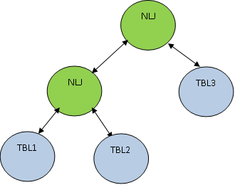
So here the first both tables are scanned and then they are joined together as per the correlation condition as TBL.ID > TBL2.ID In addition to the join method, the join order is also very important. Consider the below example: SELECT * FROM TBL1, TBL2, TBL3 WHERE TBL1.ID=TBL2.ID AND TBL2.ID=TBL3.ID; Consider that TBL1, TBL2 AND TBL3 have 10, 100 and 1000 records respectively. The condition TBL1.ID=TBL2.ID returns only 5 records, whereas TBL2.ID=TBL3.ID returns 100 records, then it’s better to join TBL1 and TBL2 first so that lesser number of records get joined with TBL3. The plan will be as shown below: PostgreSQL supports the below kind of joins: Each of these Join methods are equally useful depending on the query and other parameters e.g. query, table data, join clause, selectivity, memory etc. These join methods are implemented by most of the relational databases. Let’s create some pre-setup table and populate with some data, which will be used frequently to better explain these scan methods. In all our subsequent examples, we consider default configuration parameter unless otherwise specified specifically. Nested Loop Join (NLJ) is the simplest join algorithm wherein each record of outer relation is matched with each record of inner relation. The Join between relation A and B with condition A.ID < B.ID can be represented as below: Nested Loop Join (NLJ) is the most common joining method and it can be used almost on any dataset with any type of join clause. Since this algorithm scan all tuples of inner and outer relation, it is considered to be the most costly join operation. As per the above table and data, the following query will result in a Nested Loop Join as shown below: Since the join clause is “<”, the only possible join method here is Nested Loop Join. Notice here one new kind of node as Materialize
TIP: In case join clause is “=” and nested loop join is chosen between a relation, then it is really important to investigate if more efficient join method such as hash or merge join can be chosen by tuning configuration (e.g. work_mem but not limited to ) or by adding an index, etc. Some of the queries may not have join clause, in that case also the only choice to join is Nested Loop Join. E.g. consider the below queries as per the pre-setup data: The join in the above example is just a Cartesian product of both tables. This algorithm works in two phases: The join between relation A and B with condition A.ID = B.ID can be represented as below: As per above pre-setup table and data, the following query will result in a Hash Join as shown below: Here the hash table is created on the table blogtable2 because it is the smaller table so the minimal memory required for hash table and whole hash table can fit in memory. Merge Join is an algorithm wherein each record of outer relation is matched with each record of inner relation until there is a possibility of join clause matching. This join algorithm is only used if both relations are sorted and join clause operator is “=”. The join between relation A and B with condition A.ID = B.ID can be represented as below: The example query which resulted in a Hash Join, as shown above, can result in a Merge Join if the index gets created on both tables. This is because the table data can be retrieved in sorted order because of the index, which is one of the major criteria for the Merge Join method: So, as we see, both tables are using index scan instead of sequential scan because of which both tables will emit sorted records. PostgreSQL supports various planner related configurations, which can be used to hint the query optimizer to not select some particular kind of join methods. If the join method chosen by the optimizer is not optimal, then these configuration parameters can be switch-off to force the query optimizer to choose a different kind of join methods. All of these configuration parameters are “on” by default. Below are the planner configuration parameters specific to join methods. There are many plan related configuration parameters used for various purposes. In this blog, keeping it restricted to only join methods. These parameters can be modified from a particular session. So in-case we want to experiment with the plan from a particular session, then these configuration parameters can be manipulated and other sessions will still continue to work as it is. Now, consider the above examples of merge join and hash join. Without an index, query optimizer selected a Hash Join for the below query as shown below but after using configuration, it switches to merge join even without index: Initially Hash Join is chosen because data from tables are not sorted. In order to choose the Merge Join Plan, it needs to first sort all records retrieved from both tables and then apply the merge join. So, the cost of sorting will be additional and hence the overall cost will increase. So possibly, in this case, the total (including increased) cost is more than the total cost of Hash Join, so Hash Join is chosen. Once configuration parameter enable_hashjoin is changed to “off”, this means the query optimizer directly assign a cost for hash join as disable cost (=1.0e10 i.e. 10000000000.00). The cost of any possible join will be lesser than this. So, the same query result in Merge Join after enable_hashjoin changed to “off” as even including the sorting cost, the total cost of merge join is lesser than disable cost. Now consider the below example: As we can see above, even though the nested loop join related configuration parameter is changed to “off” still it chooses Nested Loop Join as there is no alternate possibility of any other kind of Join Method to get selected. In simpler terms, since Nested Loop Join is the only possible join, then whatever is the cost it will be always the winner (Same as I used to be the winner in 100m race if I ran alone…:-)). Also, notice the difference in cost in the first and second plan. The first plan shows the actual cost of Nested Loop Join but the second one shows the disable cost of the same. All kinds of PostgreSQL join methods are useful and get selected based on the nature of the query, data, join clause, etc. In-case the query is not performing as expected, i.e. join methods are not selected as expected then, the user can play around with different plan configuration parameters available and see if something is missing.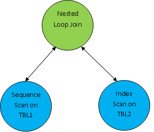
postgres=# create table blogtable1(id1 int, id2 int);

CREATE TABLE

postgres=# create table blogtable2(id1 int, id2 int);

CREATE TABLE

postgres=# insert into blogtable1 values(generate_series(1,10000),3);

INSERT 0 10000

postgres=# insert into blogtable2 values(generate_series(1,1000),3);

INSERT 0 1000

postgres=# analyze;

ANALYZENested Loop Join
For each tuple r in A
       	For each tuple s in B
            	If (r.ID < s.ID)
Emit output tuple (r,s)postgres=# explain select * from blogtable1 bt1, blogtable2 bt2 where bt1.id1 < bt2.id1;
QUERY PLAN
------------------------------------------------------------------------------
Nested Loop (cost=0.00..150162.50 rows=3333333 width=16)
Join Filter: (bt1.id1 < bt2.id1)
-> Seq Scan on blogtable1 bt1 (cost=0.00..145.00 rows=10000 width=8)
-> Materialize (cost=0.00..20.00 rows=1000 width=8)
-> Seq Scan on blogtable2 bt2 (cost=0.00..15.00 rows=1000 width=8)
(5 rows)
postgres=# explain select * from blogtable1, blogtable2;

                             QUERY PLAN

--------------------------------------------------------------------------

 Nested Loop  (cost=0.00..125162.50 rows=10000000 width=16)

   ->  Seq Scan on blogtable1  (cost=0.00..145.00 rows=10000 width=8)

   ->  Materialize  (cost=0.00..20.00 rows=1000 width=8)

      ->  Seq Scan on blogtable2  (cost=0.00..15.00 rows=1000 width=8)

(4 rows)Hash Join
postgres=# explain select * from blogtable1 bt1, blogtable2 bt2 where bt1.id1 = bt2.id1;

                               QUERY PLAN

------------------------------------------------------------------------------

 Hash Join  (cost=27.50..220.00 rows=1000 width=16)

   Hash Cond: (bt1.id1 = bt2.id1)

   ->  Seq Scan on blogtable1 bt1  (cost=0.00..145.00 rows=10000 width=8)

   ->  Hash  (cost=15.00..15.00 rows=1000 width=8)

         ->  Seq Scan on blogtable2 bt2  (cost=0.00..15.00 rows=1000 width=8)

(5 rows) Merge Join
    For each tuple r in A

        For each tuple s in B

             If (r.ID = s.ID)

                  Emit output tuple (r,s)

                  Break;

             If (r.ID > s.ID)

                  Continue;

             Else

Break;postgres=# create index idx1 on blogtable1(id1);
CREATE INDEX
postgres=# create index idx2 on blogtable2(id1);
CREATE INDEX
postgres=# explain select * from blogtable1 bt1, blogtable2 bt2 where bt1.id1 = bt2.id1;
QUERY PLAN
---------------------------------------------------------------------------------------
Merge Join (cost=0.56..90.36 rows=1000 width=16)
Merge Cond: (bt1.id1 = bt2.id1)
-> Index Scan using idx1 on blogtable1 bt1 (cost=0.29..318.29 rows=10000 width=8)
-> Index Scan using idx2 on blogtable2 bt2 (cost=0.28..43.27 rows=1000 width=8)
(4 rows)Configuration
postgres=# explain select * from blogtable1, blogtable2 where blogtable1.id1 = blogtable2.id1;

                             QUERY PLAN

--------------------------------------------------------------------------

 Hash Join  (cost=27.50..220.00 rows=1000 width=16)

   Hash Cond: (blogtable1.id1 = blogtable2.id1)

   ->  Seq Scan on blogtable1  (cost=0.00..145.00 rows=10000 width=8)

   ->  Hash  (cost=15.00..15.00 rows=1000 width=8)

      ->  Seq Scan on blogtable2  (cost=0.00..15.00 rows=1000 width=8)

(5 rows)


postgres=# set enable_hashjoin to off;

SET

postgres=# explain select * from blogtable1, blogtable2 where blogtable1.id1 = blogtable2.id1;

                             QUERY PLAN

----------------------------------------------------------------------------

 Merge Join  (cost=874.21..894.21 rows=1000 width=16)

   Merge Cond: (blogtable1.id1 = blogtable2.id1)

   ->  Sort  (cost=809.39..834.39 rows=10000 width=8)

      Sort Key: blogtable1.id1

      ->  Seq Scan on blogtable1  (cost=0.00..145.00 rows=10000 width=8)

   ->  Sort  (cost=64.83..67.33 rows=1000 width=8)

      Sort Key: blogtable2.id1

      ->  Seq Scan on blogtable2  (cost=0.00..15.00 rows=1000 width=8)

(8 rows)postgres=# explain select * from blogtable1, blogtable2 where blogtable1.id1 < blogtable2.id1;
QUERY PLAN
--------------------------------------------------------------------------
Nested Loop (cost=0.00..150162.50 rows=3333333 width=16)
Join Filter: (blogtable1.id1 < blogtable2.id1)
-> Seq Scan on blogtable1 (cost=0.00..145.00 rows=10000 width=8)
-> Materialize (cost=0.00..20.00 rows=1000 width=8)
-> Seq Scan on blogtable2 (cost=0.00..15.00 rows=1000 width=8)
(5 rows)
postgres=# set enable_nestloop to off;
SET
postgres=# explain select * from blogtable1, blogtable2 where blogtable1.id1 < blogtable2.id1;
QUERY PLAN
--------------------------------------------------------------------------
Nested Loop (cost=10000000000.00..10000150162.50 rows=3333333 width=16)
Join Filter: (blogtable1.id1 < blogtable2.id1)
-> Seq Scan on blogtable1 (cost=0.00..145.00 rows=10000 width=8)
-> Materialize (cost=0.00..20.00 rows=1000 width=8)
-> Seq Scan on blogtable2 (cost=0.00..15.00 rows=1000 width=8)
(5 rows)Conclusion