blog
Monitoring Galera Cluster for MySQL or MariaDB – Understanding Metrics (Updated)

To operate any database efficiently, you need to have insight into database performance. This might not be obvious when everything is going well, but as soon as something goes wrong, access to information can be instrumental in quickly and correctly diagnosing the problem.
All databases make some of their internal status data available to users. In MySQL, you can get this data mostly by running ‘SHOW STATUS‘ and ‘SHOW GLOBAL STATUS‘, by executing ‘SHOW ENGINE INNODB STATUS‘, checking information_schema tables and, in newer versions, by querying performance_schema tables.
These methods are far from convenient in day-to-day operations, hence the popularity of different monitoring and trending solutions. Tools like Nagios/Icinga are designed to watch hosts/services, and alert when a service falls outside an acceptable range. Other tools such as Cacti and Munin provide a graphical look at host/service information, and give historical context to performance and usage. ClusterControl combines these two types of monitoring, so we’ll have a look at the information it presents, and how we should interpret it.
If you’re using Galera Cluster (MySQL Galera Cluster by Codership or MariaDB Cluster or Percona XtraDB Cluster), you may have noticed the following section in ClusterControl’s “Overview” tab:
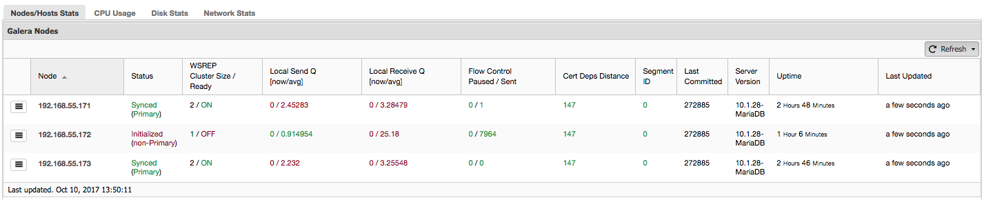
Let’s see, step by step, what kind of data we have here.
The first column contains the list of nodes with their IP addresses – there’s not much else to say about it.
Second column is more interesting – it describes node status (wsrep_local_state_comment status). A node can be in different states:
- Initialized – The node is up and running, but it’s not a part of a cluster. It can be caused, for example, by network issues;
- Joining – The node is in the process of joining the cluster and it’s either receiving or requesting a state transfer from one of other nodes;
- Donor/Desynced – The node serves as a donor to some other node which is joining the cluster;
- Joined – The node is joined the cluster but its busy catching up on committed write sets;
- Synced – The node is working normally.
In the same column within the bracket is the cluster status (wsrep_cluster_status status). It can have three distinct states:
- Primary – The communication between nodes is working and quorum is present (majority of nodes is available)
- Non-Primary – The node was a part of the cluster but, for some reason, it lost contact with the rest of the cluster. As a result, this node is considered inactive and it won’t accept queries
- Disconnected – The node could not establish group communication.
“WSREP Cluster Size / Ready” tells us about a cluster size as the node sees it, and whether the node is ready to accept queries. Non-Primary components create a cluster with size of 1 and wsrep readiness is OFF.
Let’s take a look at the screenshot above, and see what it is telling us about Galera. We can see three nodes. Two of them (192.168.55.171 and 192.168.55.173) are perfectly fine, they are both “Synced” and the cluster is in “Primary” state. The cluster currently consists of two nodes. Node 192.168.55.172 is “Initialized” and it forms “non-Primary” component. It means that this node lost connection with the cluster – most likely some kind of network issues (in fact, we used iptables to block a traffic to this node from both 192.168.55.171 and 192.168.55.173).
At this moment we have to stop a bit and describe how Galera Cluster works internally. We’ll not go into too much details as it is not within a scope of this blog post but some knowledge is required to understand the importance of the data presented in next columns.
Galera is a “virtually” synchronous, multi-master cluster. It means that you should expect data to be transferred across nodes “virtually” at the same time (no more annoying issues with lagging slaves) and that you can write to any node in a cluster (no more annoying issues with promoting a slave to master). To accomplish that, Galera uses writesets – atomic set of changes that are replicated across the cluster. A writeset can contain several row changes and additional needed information like data regarding locking.
Once a client issues COMMIT, but before MySQL actually commits anything, a writeset is created and sent to all nodes in the cluster for certification. All nodes check whether it’s possible to commit the changes or not (as changes may interfere with other writes executed, in the meantime, directly on another node). If yes, data is actually committed by MySQL, if not, rollback is executed.
What’s important to remember is the fact that nodes, similar to slaves in regular replication, may perform differently – some may have better hardware than others, some may be more loaded than others. Yet Galera requires them to process the writesets in a short and quick manner, in order to maintain “virtual” synchronization. There has to be a mechanism which can throttle the replication and allow slower nodes to keep up with the rest of the cluster.
Let’s take a look at “Local Send Q [now/avg]” and “Local Receive Q [now/avg]” columns. Each node has a local queue for sending and receiving writesets. It allows to parallelize some of the writes and queue data which couldn’t be processed at once if node cannot keep up with traffic. In SHOW GLOBAL STATUS we can find eight counters describing both queues, four counters per queue:
- wsrep_local_send_queue – current state of the send queue
- wsrep_local_send_queue_min – minimum since FLUSH STATUS
- wsrep_local_send_queue_max – maximum since FLUSH STATUS
- wsrep_local_send_queue_avg – average since FLUSH STATUS
- wsrep_local_recv_queue – current state of the receive queue
- wsrep_local_recv_queue_min – minimum since FLUSH STATUS
- wsrep_local_recv_queue_max – maximum since FLUSH STATUS
- wsrep_local_recv_queue_avg – average since FLUSH STATUS
The above metrics are unified across nodes under ClusterControl -> Performance -> DB Status:
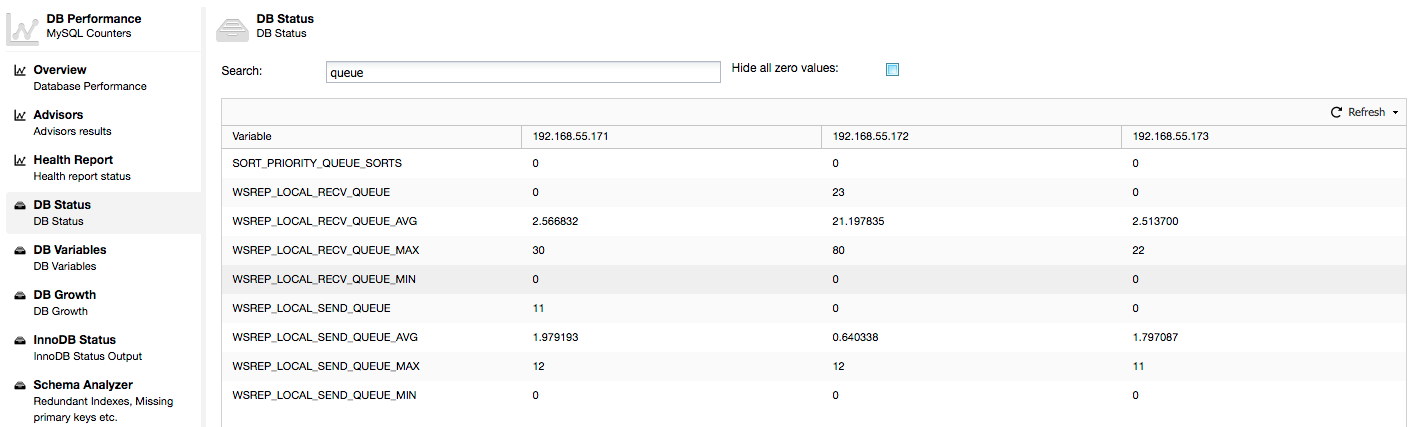
ClusterControl displays “now” and “average” counters, as they are the most meaningful as a single number (you can also create custom graphs based on variables describing the current state of the queues) . When we see that one of the queues is rising, this means that the node can’t keep up with the replication and other nodes will have to slow down to allow it to catch up. We’d recommend to investigate a workload of that given node – check the process list for some long running queries, check OS statistics like CPU utilization and I/O workload. Maybe it’s also possible to redistribute some of the traffic from that node to the rest of the cluster.
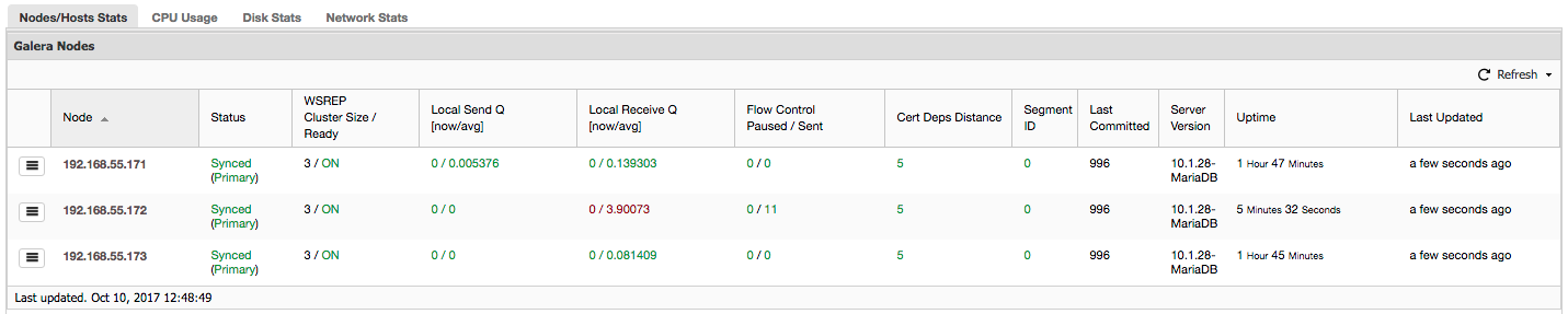
“Flow Control Paused” shows information about the percentage of time a given node had to pause its replication because of too heavy load. When a node can’t keep up with the workload it sends Flow Control packets to other nodes, informing them they should throttle down on sending writesets. In our screenshot, we have value of ‘0.30’ for node 192.168.55.172. This means that almost 30% of the time this node had to pause the replication because it wasn’t able to keep up with writeset certification rate required by other nodes (or simpler, too many writes hit it!). As we can see, it’s “Local Receive Q [avg]” points us also to this fact.
Next column, “Flow Control Sent” gives us information about how many Flow Control packets a given node sent to the cluster. Again, we see that it’s node 192.168.55.172 which is slowing down the cluster.
What can we do with this information? Mostly, we should investigate what’s going on in the slow node. Check CPU utilization, check I/O performance and network stats. This first step helps to assess what kind of problem we are facing.
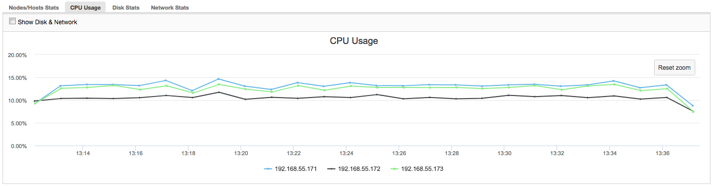
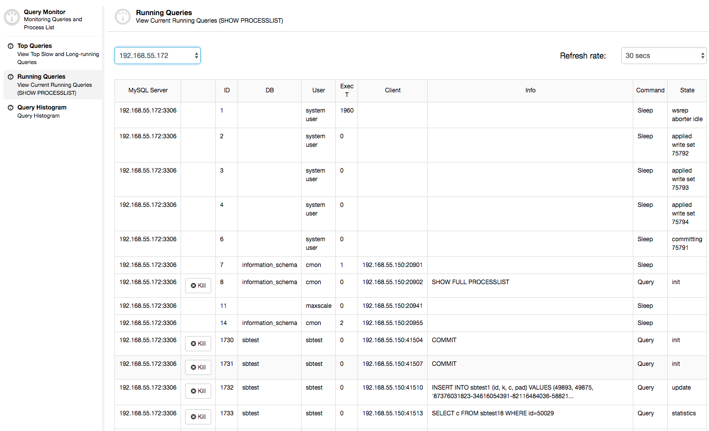
In this case, once we switch to CPU Usage tab, it becomes clear that extensive CPU utilization is causing our issues. Next step would be to identify the culprit by looking into PROCESSLIST (Query Monitor -> Running Queries -> filter by 192.168.55.172) to check for offending queries:
Or, check processes on the node from operating system’s side (Nodes -> 192.168.55.172 -> Top) to see if the load is not caused by something outside of Galera/MySQL.
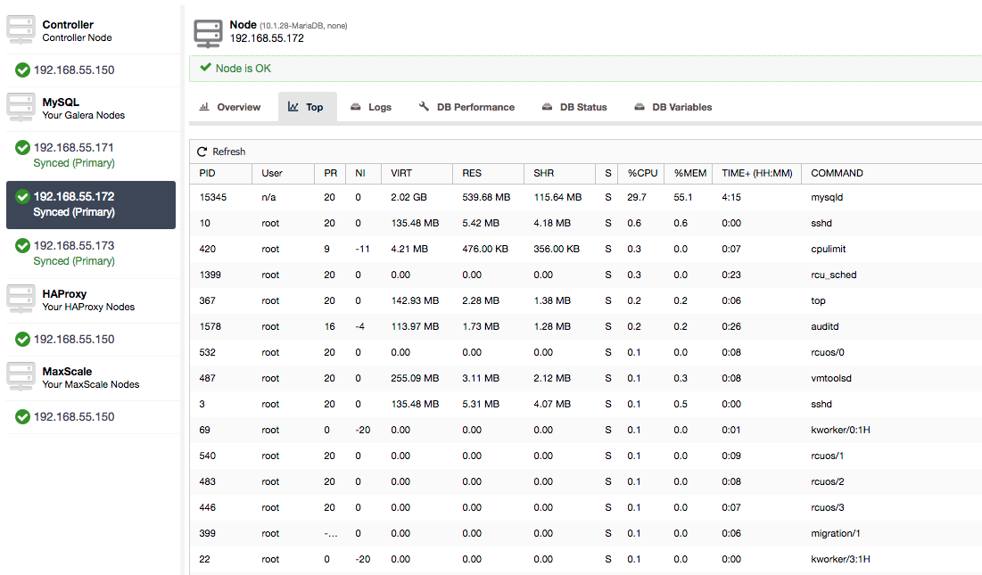
In this case, we have executed mysqld command through cpulimit, to simulate slow CPU usage specifically for mysqld process by limiting it to 30% out of 400% available CPU (the server has 4 cores).
“Cert Deps Distance” column gives us information about how many writesets, on average, can be applied in parallel. Writesets can, sometimes, be executed at the same time – Galera takes advantage of this by using multiple wsrep_slave_threads to apply writesets. This column gives you some idea how many slave threads you could use on your workload. It’s worth noting that there’s no point in setting up wsrep_slave_threads variable to values higher than you see in this column or in wsrep_cert_deps_distance status variable, on which “Cert Deps Distance” column is based. Another important note – there is no point either in setting wsrep_slave_threads variable to more than number of cores your CPU has.
“Segment ID” – this column will require some more explanation. Segments are a new feature added in Galera 3.0. Before this version, writesets were exchanged between all nodes. Let’s say we have two datacenters:
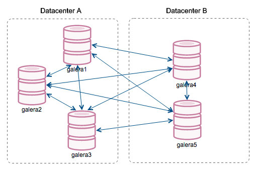
This kind of chatter works ok on local networks but WAN is a different story – certification slows down due to increased latency, additional costs are generated because of network bandwidth used for transferring writesets between every member of the cluster.
With the introduction of “Segments”, things changed. You can assign a node to a segment by modifying wsrep_provider_options variable and adding “gmcast.segment=x” (0, 1, 2) to it. Nodes with the same segment number are treated as they are in the same datacenter, connected by local network. Our graph then becomes different:
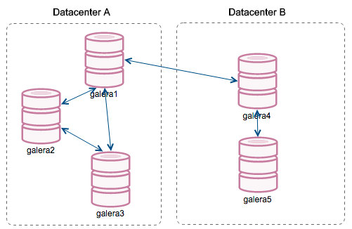
The main difference is that it’s no more everyone to everyone communication. Within each segment, yes – it’s still the same mechanism but both segments communicate only through a single connection between two chosen nodes. In case of downtime, this connection will failover automatically. As a result, we get less network chatter and less bandwidth usage between remote datacenters. So, basically, “Segment ID” column tells us to which segment a node is assigned.
“Last Committed” column gives us information about the sequence number of the writeset that was last executed on a given node. It can be useful in determining which node is the most current one if there’s a need to bootstrap the cluster.
Rest of the columns are self-explanatory: Server version, uptime of a node and when the status was updated.
As you can see, the “Galera Nodes” section of the “Nodes/Hosts Stats” in the “Overview” tab gives you a pretty good understanding of the cluster’s health – whether it forms a “Primary” component, how many nodes are healthy, are there any performance issues with some nodes and if yes, which node is slowing down the cluster.
This set of data comes in very handy when you operate your Galera cluster, so hopefully, no more flying blind 🙂