Introduction to MariaDB Vector Search

Vector search is now entering your RDBMs, providing enhanced capabilities in a familiar interface. MariaDB introduced native vector search capabilities in its 11.8 release, which is the current Long-Term Support (LTS) release for these features. Vector search is fundamentally different from traditional search with its focus on semantic similarity through numerical representations of data. And with that comes important nuances.

In this blog post, we are going to look into the differences between traditional and vector search, introduce and demonstrate core concepts using a simple 2-dimensional example, before demonstrating a real-world application using a 384-dimensional vector created by an AI model to perform semantic similarity queries for finding relevant products, showcasing how vector search retrieves items based on meaning rather than just keyword matching.

MariaDB vector search compared to traditional search

The main difference between the two lies in what you are searching for and how relevance is determined.

Feature	MariaDB Traditional Search	MariaDB Vector Search
Goal	Find exact matches or matches based on keywords, prefixes, or full-text relevance.	Find items similar in meaning or context to a query, even if the exact keywords are different.
Data Type	Standard data types: INT, VARCHAR, TEXT, DATETIME, etc.	VECTOR(N) data type, where N is the dimension (e.g., VECTOR(384)).
Search Mechanism	Uses B-Tree indexes, Full-Text indexes (FULLTEXT), or simple equality/LIKE operators.	Uses Approximate Nearest Neighbor (ANN) index (specifically a modified Hierarchical Navigable Small World, or HNSW, in MariaDB).
Relevance/Similarity	Based on lexical or structural matching (e.g., word count, frequency, keyword presence).	Based on geometric distance (e.g., Euclidean distance or Cosine similarity) in a high-dimensional space.
Query Example	SELECT * FROM products WHERE name LIKE ‘red car%’; or …MATCH(description) AGAINST(‘toy’);	SELECT * FROM products ORDER BY VEC_DISTANCE_COSINE(embedding, <query_vector>) LIMIT K;
Output	Exact or keyword-relevant results.	Semantic results (“show me things like X”).
Use Case	Inventory lookup, filtering by category, finding documents containing specific words.	Semantic similarity search, recommendation engines, reverse image search, finding similar documents/products/music.

The following are functions that can be used for vector search, see MariaDB Vector Functions for reference :

• VEC_FromText()
• VEC_DISTANCE()
• VEC_DISTANCE_COSINE()
• VEC_DISTANCE_EUCLIDEAN()

There are related variables called Modified Hierarchical Navigable Small World (MHNSW), prefixed with “mhnsw_”.

MariaDB [(none)]> show variables like '%mhnsw%';
+------------------------+-----------+
| Variable_name          | Value     |
+------------------------+-----------+
| mhnsw_default_distance | euclidean |
| mhnsw_default_m        | 6         |
| mhnsw_ef_search        | 20        |
| mhnsw_max_cache_size   | 16777216  |
+------------------------+-----------+

Tuning parameters like mhnsw_default_m and mhnsw_ef_search balance accuracy and performance. For example, set mhnsw_default_m=200 (maximum), provides better accuracy, but larger index size and slower updates and searches. As you can imagine, vector search introduces differences that will affect how you index and query your database, as well as the kind of results you can expect. Let’s consider why and look at how this works in action.

MariaDB vector search, embedding, indexing, and function specifics

Vector search is basically finding similar items according to relationships between their vectors or embeddings, i.e. their data converted into numerical representations. The more vectors (dimensions), the more accurately semantic your data can be queried. Machine learning embeddings often have dimensions ranging from 150 to 1536, or even higher. We’ll showcase a 384-dimensional vector later; but let’s start with a smaller one using a 2-number vector.

Imagine we have a toy shop and want to categorize our toys along two dimensions, hardness and price:

• vector[0] = hardness (0 = soft, 1 = hard)
• vector[1] = price (0 = cheap, 1 = expensive)

We’ll index our dataset using Euclidean distance because it’s the most intuitive for our little 2-dimensional map:

CREATE TABLE toys (
  id INT PRIMARY KEY AUTO_INCREMENT,
  name VARCHAR(50) NOT NULL,
  embedding VECTOR(2) NOT NULL,
  VECTOR INDEX (embedding) DISTANCE=euclidean
);

Let’s add the following rows into the table:

INSERT INTO toys (name, embedding) VALUES
  ('Teddy Bear',    VEC_FromText('[0.05, 0.20]')),  -- soft & cheap-ish
  ('Plush Unicorn', VEC_FromText('[0.10, 0.30]')),  -- soft & a bit pricier
  ('Wooden Blocks', VEC_FromText('[0.70, 0.25]')),
  ('Toy Car',       VEC_FromText('[0.85, 0.45]')),
  ('Board Game',    VEC_FromText('[0.60, 0.35]')),
  ('Robot Kit',     VEC_FromText('[0.95, 0.90]')),  -- hard & expensive
  ('Dollhouse',     VEC_FromText('[0.50, 0.80]')),
  ('Puzzle',        VEC_FromText('[0.55, 0.20]')),
  ('Water Gun',     VEC_FromText('[0.90, 0.25]')),
  ('RC Drone',      VEC_FromText('[0.98, 0.95]'));  -- very hard & very expensive

If we do a simple SELECT * statement, we’ll see the following gibberish embedding output in our terminal:

MariaDB [toyshop]> SELECT * FROM toys;
+----+---------------+-----------+
| id | name          | embedding |
+----+---------------+-----------+
|  1 | Teddy Bear    | ��L=��L>  |
|  2 | Plush Unicorn | ���=���>  |
|  3 | Wooden Blocks | 333?  �>  |
|  4 | Toy Car       | ��Y?ff�>  |
|  5 | Board Game    | ��?33�>  |
|  6 | Robot Kit     | 33s?fff?  |
|  7 | Dollhouse     |    ?��L?  |
|  8 | Puzzle        | ��
                         ?��L>  |
|  9 | Water Gun     | fff?  �>  |
| 10 | RC Drone      | H�z?33s?  |
+----+---------------+-----------+

The vector embedding values are not displayed in a human-readable form. We have to use a function called VEC_ToText to convert the vector datatype to text:

MariaDB [toyshop]> SELECT id,name,VEC_ToText(embedding) FROM toys;
+----+---------------+-----------------------+
| id | name          | VEC_ToText(embedding) |
+----+---------------+-----------------------+
|  1 | Teddy Bear    | [0.05,0.2]            |
|  2 | Plush Unicorn | [0.1,0.3]             |
|  3 | Wooden Blocks | [0.7,0.25]            |
|  4 | Toy Car       | [0.85,0.45]           |
|  5 | Board Game    | [0.6,0.35]            |
|  6 | Robot Kit     | [0.95,0.9]            |
|  7 | Dollhouse     | [0.5,0.8]             |
|  8 | Puzzle        | [0.55,0.2]            |
|  9 | Water Gun     | [0.9,0.25]            |
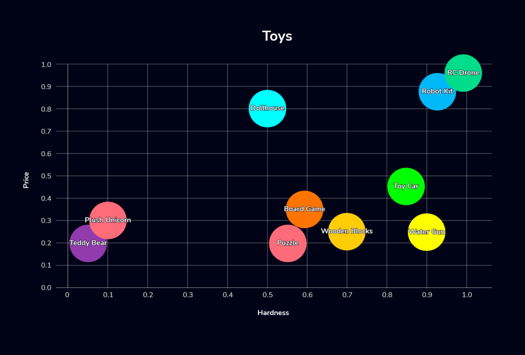
| 10 | RC Drone      | [0.98,0.95]           |
+----+---------------+-----------------------+

We can visually represent the records above using the following 2-dimensional bubble chart:

We can then use the SQL query to perform a vector search for toys that are soft and cheap (soft is represented with x approaching 0 and cheap is represented with y approaching 0). In this example, we define soft as hardness=0.05 and cheap as price=0.15, and we want to find the top 5 toys in our collection that meet these criteria:

SELECT name AS soft_n_cheap
FROM toys
ORDER BY VEC_DISTANCE_EUCLIDEAN(embedding, VEC_FromText('[0.05, 0.15]'))
LIMIT 5;
+---------------+
| soft_n_cheap  |
+---------------+
| Teddy Bear    |
| Plush Unicorn |
| Puzzle        |
| Board Game    |
| Wooden Blocks |
+---------------+

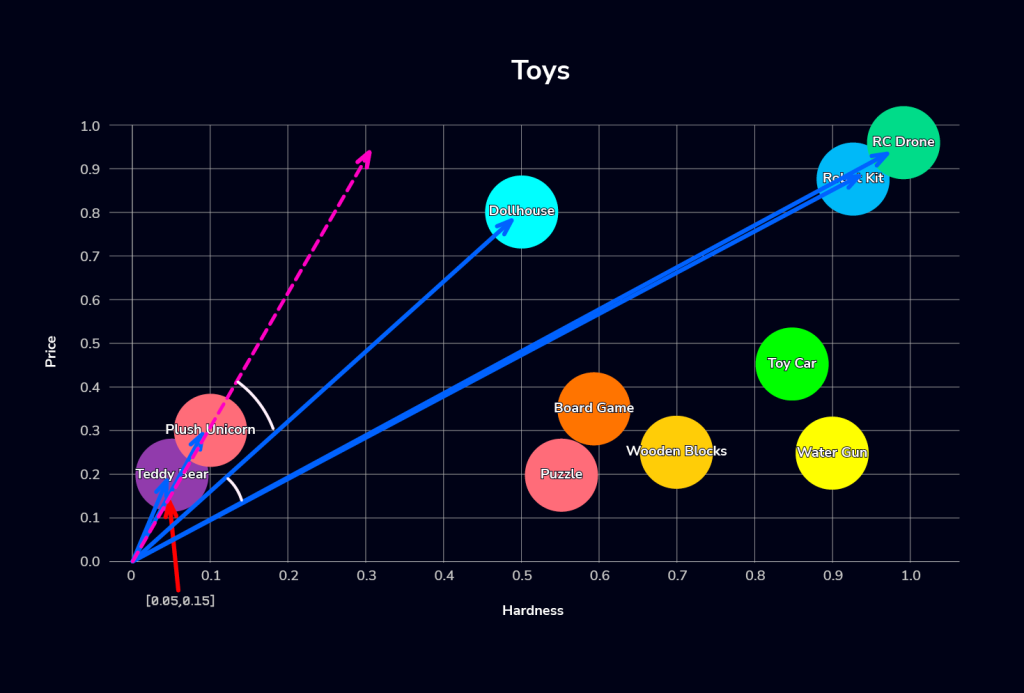
We use the VEC_DISTANCE_EUCLIDEAN function to find the nearest toys to x=0.05 and y=0.15, visualized thusly:

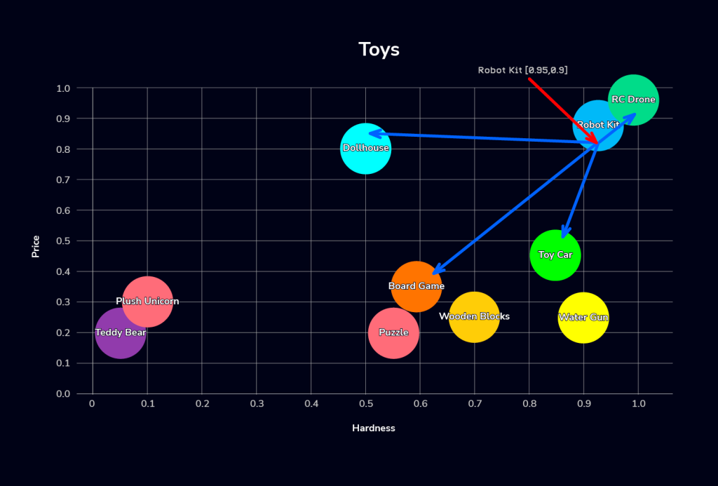
Now, let’s try to find toys on the opposite end, with characteristics similar to the “Robot Kit” (hard and pricey):

SELECT t.name AS similar_to_robotkit
FROM toys AS t
JOIN toys AS seed ON seed.name = 'Robot Kit'
ORDER BY VEC_DISTANCE_EUCLIDEAN(t.embedding, seed.embedding)
LIMIT 5;
+---------------------+
| similar_to_robotkit |
+---------------------+
| Robot Kit           |
| RC Drone            |
| Toy Car             |
| Dollhouse           |
| Board Game          |
+---------------------+

Again, we use the VEC_DISTANCE_EUCLIDEAN function, but to find the nearest toys to x=0.95 and y=0..9:

MariaDB supports another vector function called VEC_DISTANCE_COSINE, i.e. cosine similarity. We can even query the table utilizing cosine similarity for ordering although our current index relies on Euclidean distance (which may result in slower lookups as the data set grows). Using the cosine similarity function yields a different result set:

SELECT name AS soft_n_cheap
FROM toys
ORDER BY VEC_DISTANCE_COSINE(embedding, VEC_FromText('[0.05, 0.15]'))
LIMIT 5;
+---------------+
| soft_n_cheap  |
+---------------+
| Plush Unicorn |
| Teddy Bear    |
| Dollhouse     |
| RC Drone      |
| Robot Kit     |
+---------------+

Why? We’ll get into the details below; but, this is simply because the cosine distance function compares vectors based on the angle to the defined query coordinates, which is represented here as [0.05, 0.15]. This coordinate signifies all toys with a similar ratio of 0.05 hardness to 0.15 priceyness, as depicted below:

Now that we’ve covered the basics, let’s detail two core functions and their impact on indexing and results.

Euclidean distance vs cosine similarity specifics

Euclidean distance measures the straight-line distance between two points, answering “How far apart are these two dots?” Conversely, cosine similarity focuses on the angle between two vectors, essentially asking, “Are these two pointing in the same direction?” Here is a quick rule of thumb to help you decide which method to employ:

• Use Euclidean when actual values matter, e.g. you care that one toy is truly pricier/harder.
• Use Cosine when direction / composition matters and scale shouldn’t (typical for embeddings).

Selecting between euclidean distance and cosine similarity metrics is a crucial initial step when creating a table for MariaDB Vector Search. This choice fundamentally impacts how the data is stored, affecting the speed and efficiency of subsequent data storage operations. Since this determination must be made upon table creation, failing to choose the correct metric initially will necessitate an ALTER TABLE operation later on.

We know their high-level differences, e.g. distance vs. angle / orientation, and when to use one method over the other, let’s go back to our example use case to see how each method would affect result generation:

Embeddings

• embedding[0] = hardness (0 soft → 1 hard)
• embedding[1] = price (0 cheap → 1 expensive)

Searching for “soft & cheap” items (coordinates of 0.05 hardness and 0.15 pricey), Euclidean distance favors toys closest to this exact coordinate (very soft, very cheap), such as the Teddy Bear and Plush Unicorn. This search process can be imagined as an expanding circle from the query coordinates, as shown by the green gradient circle.

Meanwhile, cosine similarity prioritizes items with a similar ratio, such as softness-to-price. Therefore, a slightly more expensive item could rank higher if its ratio is closer relative to the others, pulling in items like a Dollhouse instead of others that may be closer in absolute price or softness. This concept is visualized by the gradient rectangle below:

Comparing the two results, you see that the Teddy Bear, Plush Unicorn, and Dollhouse are considered equally similar to the query vector (hardness=0.05, price=0.15) using cosine similarity, as their angles relative to the query point are the closest. But, the Dollhouse is ranked worse using euclidean distance because its distance is greater.

The above example is just a simple vehicle to demonstrate the concepts; now, let’s look at a real-world use case. 

Creating vector embeddings at scale using an AI model

In our example above, we define our own simple vector embeddings with 2 vectors (price and hardness). Smaller vectors (lower dimensions) are more efficient to keep in memory or to process, while bigger vectors (higher dimensions) capture complex relationships, but are prone to overfitting. For reference, the GPT-2 model family has an embedding size of at least 768. In the following example, we’ll create a more accurate toy inventory with 384 vectors, which we’ll use with the help of an AI model. 

First, we have to set up our preferred AI model to generate vector embeddings, e.g., OpenAI, Claude, etc. We’ll use Sentence Transformers by Hugging Face for sentence, text and image embeddings. Since this is a large language model (LLM) application, cosine similarity is the better choice because it focuses on the semantic meaning (direction) of embeddings rather than their magnitude.

Install our the required tools:

apt install -y libmariadb-dev

pip install -U sentence-transformers mariadb

This example utilizes a Python script, toy_vectors.py (available at here), to handle several tasks like generation of sample data, and execution of a vector search query.

Install MariaDB 11.8 and later, and create a database called toyshop with the associated user:

MariaDB> CREATE DATABASE toyshop;
MariaDB> CREATE USER toyshop IDENTIFIED BY 'pass123';
MariaDB> GRANT ALL PRIVILEGES ON toyshop.* TO toyshop@localhost;

We will now generate a test data set containing 50 toy entries. Please note that the toy names and descriptions are created from a limited, pre-defined word list, so the resulting text should not be interpreted as having real semantic meaning:

$ python3 toy_vectors.py --host localhost --user toyshop --password 'pass123' --database toyshop --init
Loading embedding model: sentence-transformers/all-MiniLM-L6-v2 ...
Creating schema and inserting 50 toys ...
Done loading toys.

For reference, this is the table definition created by the script:

CREATE TABLE `toys` (
  `toy_id` bigint(20) NOT NULL AUTO_INCREMENT,
  `name` varchar(120) NOT NULL,
  `description` text NOT NULL,
  `embedding` vector(384) NOT NULL,
  PRIMARY KEY (`toy_id`),
  UNIQUE KEY `uniq_name` (`name`),
  VECTOR KEY `embedding` (`embedding`) `DISTANCE`=cosine
);

This is what a row looks like in the table with 384 embeddings:

MariaDB [toyshop]> SELECT toy_id,name,description,VEC_ToText(embedding) from toys limit 1\G
*************************** 1. row ***************************
               toy_id: 1
                 name: Wooden Teddy Bear #1

          description: A wooden teddy bear for outdoor play. Built to last.
VEC_ToText(embedding): [-0.00415802,0.0486636,0.0931525,0.0335656,-0.0225082,0.0405051,0.0611988,0.00668925,0.0318281,0.113786,-0.0528246,0.0293252,-0.0170199,0.0194476,0.0269966,0.00319623,0.0023232,0.0252253,0.065384,-0.059229,-0.0790046,0.017883,-0.026427,0.0126928,-0.0333909,0.0286699,-0.0369491,-0.0270459,0.044531,-0.0550842,0.0157583,-0.06999,0.046131,0.0147048,-0.0714118,0.0681623,0.0188634,-0.0893993,0.0114057,0.0188946,-0.0154973,0.0559293,0.0524786,0.0465031,-0.0175183,0.0249896,-0.06199,-0.0615214,0.0428483,0.0230578,-0.00937421,-0.0304126,-0.0277833,-0.00158542,-0.00245011,-0.0465182,0.0122023,-0.0344862,0.0503625,0.0324417,0.00258765,0.041926,0.0767669,0.00974742,-0.0106992,-0.0262717,-0.0902694,-0.0150526,0.0103858,0.0213565,0.0159495,0.0758756,0.0231532,-0.0268869,-0.0454534,-0.0706498,-0.012939,-0.0474217,0.084309,0.0420658,-0.0862658,0.024764,-0.00940316,-0.057419,-0.01943,0.0219899,0.00237197,0.0485456,-0.0871049,-0.00127116,-0.0283014,-0.00862217,-0.0159227,0.0678336,-0.0319935,0.00216475,0.0149419,-0.00147688,-0.0137513,0.0220396,-0.000944182,0.0252996,0.0968739,-0.0221802,0.0199244,-0.0651055,-0.0977446,0.0413534,0.024373,0.032323,-0.0932603,-0.0398666,-0.035713,0.0251915,-0.0576673,-0.0108505,-0.0349105,0.0220615,0.00249579,-0.0104649,0.11406,0.0199797,-0.0178575,0.0327065,-0.059112,-0.0523251,0.107924,-3.19871e-33,0.0615152,-0.0805271,0.0290496,0.043726...

Let’s now submit a few queries. For every query, the script will execute the following steps:

1. Load the chosen embedding AI model into memory.
2. Convert the “–query” value into an embedding vector using the loaded AI model.
3. Perform SQL query onto the MariaDB table with VEC_DISTANCE_COSINE ordering.
4. MariaDB returns the toy_id, name, description, and embedding columns to the script.
5. The script calculates the distance between the “query” vector embedding versus the value of embedding column for every tuple returned by MariaDB
6. The script presents the final output (toy name, id, distance, description) to the user

For our first query, let’s search for toys that are “soft cuddly bear for bedtime”:

$ python3 toy_vectors.py --host 127.0.0.1 --user toyshop --password 'pass123' --database toyshop --query "soft cuddly bear for bedtime" --topk 5
Loading embedding model: sentence-transformers/all-MiniLM-L6-v2 ...

Query: soft cuddly bear for bedtime

1. Wooden Teddy Bear #1 (id=1)  dist=0.4897
   A wooden teddy bear for outdoor play. Built to last.

2. Waterproof Teddy Bear #40 (id=40)  dist=0.5387
   A waterproof teddy bear for preschoolers. No small parts.

3. Classic Teddy Bear #49 (id=49)  dist=0.5622
   A classic teddy bear for STEM learning. Travel friendly.

4. Eco-Friendly Teddy Bear #39 (id=39)  dist=0.5735
   A eco-friendly teddy bear for STEM learning. No small parts.

5. Cuddly Dollhouse #15 (id=15)  dist=0.5967
   A cuddly dollhouse for outdoor play. Easy to clean.

Notice anything about the results above? Not many would fit our definition of “soft cuddly bear for bedtime.” Where a traditional query might return zero results because it’s looking for presence, a vector similarity one will always return a result because it’s looking for relevance according to your selected function — sometimes resulting in confounding results.

Standard database design best practices apply, some maybe even more so here; but, the advantage of a database like MariaDB is that you can perform hybrid search, combining keyword and vector similarity search in the same query. From there, it combines and re-ranks the results using algorithms like Reciprocal Rank Fusion (RRF) for improved accuracy.  

But, let’s stay with similarity search for now; here’s another query to find toys for my preschool twin:

$ python3 toy_vectors.py --host 127.0.0.1 --user toyshop --password 'pass123' --database toyshop --query "for my preschool twin" --topk 5
Loading embedding model: sentence-transformers/all-MiniLM-L6-v2 ...

Query: for my preschool twin

1. Waterproof Teddy Bear #40 (id=40)  dist=0.4484
   A waterproof teddy bear for preschoolers. No small parts.

2. Plush Play Kitchen #10 (id=10)  dist=0.4946
   A plush play kitchen for preschoolers. No small parts.

3. Plush Kite #43 (id=43)  dist=0.5103
   A plush kite for kids 6+. Encourages imagination.

4. Durable Craft Set #35 (id=35)  dist=0.5104
   A durable craft set for toddlers. Bright colors.

5. Magnetic Kite #12 (id=12)  dist=0.5148

   A magnetic kite for preschoolers. Parent-approved fun.

And here’s one more example that returns more relevant results to search for electronics for my teenage son:

$ python3 toy_vectors.py --host 127.0.0.1 --user toyshop --password 'pass123' --database toyshop --query "electronics for my teenage son" --topk 5
Loading embedding model: sentence-transformers/all-MiniLM-L6-v2 ...

Query: electronics for my teenage son

1. Lightweight Robot Kit #42 (id=42)  dist=0.5711
   A lightweight robot kit for preschoolers. Quick to set up.

2. Musical Robot Kit #23 (id=23)  dist=0.5968
   A musical robot kit for family game night. Includes instructions.

3. Portable Toy Car #46 (id=46)  dist=0.5985
   A portable toy car for outdoor play. Parent-approved fun.

4. Soft Robot Kit #4 (id=4)  dist=0.5989
   A soft robot kit for family game night. Built to last.

5. Waterproof Robot Kit #29 (id=29)  dist=0.6076
   A waterproof robot kit for toddlers. Easy to clean.

We can also use the standard SQL text matching query against the table:

MariaDB [toyshop]> SELECT * FROM toyshop WHERE Description like '%toy car%' LIMIT 10;
+--------+----------------------+
| toy_id | name                 |
+--------+----------------------+
|      9 | Colorful Toy Car #9  |
|     18 | Mini Toy Car #18     |
|     24 | Classic Toy Car #24  |
|     46 | Portable Toy Car #46 |
+--------+----------------------+

The query only returned four rows, despite the requested limit of ten, which suggests that no further results could be found through lexical matching. Furthermore, this query is not optimized for the table because the “Description” column used in the WHERE clause is not indexed, which would lead to slower performance with a larger dataset.

Wrapping up

MariaDB 11.8 introduced MariaDB Vector Search, enabling efficient similarity search directly within your database. This feature addresses the general need to store and retrieve vectors based on a distance function without adding the complexity that comes with incorporating an additional database to your stack, flattening your learning curve and simplifying ops.

ClusterControl further simplifies its operations by enabling you to place your database where you want and unify day 2 ops across your preferred architecture, be it on-prem, multi-cloud, or hybrid. If you haven’t yet, try it free for 30 days by following the instructions below.

Install ClusterControl in 10-minutes. Free 30-day Enterprise trial included!

Script Installation Instructions

The installer script is the simplest way to get ClusterControl up and running. Run it on your chosen host, and it will take care of installing all required packages and dependencies.

Offline environments are supported as well. See the Offline Installation guide for more details.

On the ClusterControl server, run the following commands:

wget https://severalnines.com/downloads/cmon/install-cc
chmod +x install-cc

With your install script ready, run the command below. Replace S9S_CMON_PASSWORD and S9S_ROOT_PASSWORD placeholders with your choice password, or remove the environment variables from the command to interactively set the passwords. If you have multiple network interface cards, assign one IP address for the HOST variable in the command using HOST=<ip_address>.

S9S_CMON_PASSWORD=<your_password> S9S_ROOT_PASSWORD=<your_password> HOST=<ip_address> ./install-cc # as root or sudo user

After the installation is complete, open a web browser, navigate to https://<ClusterControl_host>/, and create the first admin user by entering a username (note that “admin” is reserved) and a password on the welcome page. Once you’re in, you can deploy a new database cluster or import an existing one.

The installer script supports a range of environment variables for advanced setup. You can define them using export or by prefixing the install command.

See the list of supported variables and example use cases to tailor your installation.

Other Installation Options

Helm Chart

Deploy ClusterControl on Kubernetes using our official Helm chart.

Ansible Role

Automate installation and configuration using our Ansible playbooks.

Puppet Module

Manage your ClusterControl deployment with the Puppet module.

ClusterControl on Marketplaces

Prefer to launch ClusterControl directly from the cloud? It’s available on these platforms:

• DigitalOcean Marketplace
• gridscale.io Marketplace
• Vultr Marketplace
• Linode Marketplace
• Google Cloud Platform