blog
Monitoring Host Metrics of Your Database Instances – How to Interpret Operating System Data

Monitoring the metrics of the database hosts is critical. By keeping Swap and Physical Memory usage within allowable limits, you’ll ensure that there is enough memory for queries to be executed and connections to be created. By monitoring Disk Utilization, you can map growth patterns and better plan for capacity upgrades. If you’re using ClusterControl, you would have seen metrics like CPU utilization, Disk, Network Interface , Swap memory usage, physical memory usage, free physical memory, processes and event logs.
In this blog, we will discuss generic host statistics – CPU, disk, network and memory and the meaning of the data. This is a follow-up to an earlier blog post on Galera metrics monitoring, where we covered the different WSREP variables and how to determine whether cluster members are able to catch up with certifying and applying of write-sets.
So let’s have a look at these metrics. Below is a screenshot of the “Hosts” section of the ClusterControl Overview tab.
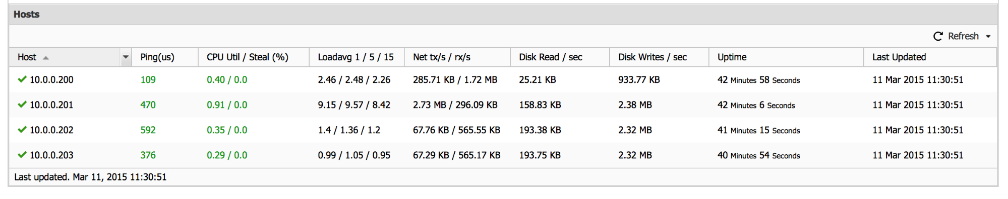
What we can see here is some basic information on node health. Ping (shown here in microseconds) can be useful in catching up some network issues or cases when a node is so overloaded that it cannot keep up with network requests. It can also give you some estimation on maximum possible Galera performance – write-set certification requires the write-set to be transferred to all nodes to check if it can be committed to the cluster. This basically sets a very strict limitation, known also as a Callaghan’s Law: “a given row can’t be modified more than once per RTT”. As long as modifications are split across many rows, network latency is not that problematic – it adds to the given DML’s latency, but, in the meantime, the application can execute queries which access and modify other parts of the database – those queries can execute in parallel, and they won’t be affected by a RTT length. The problem begins to show up when some of the rows are more frequently modified and hotspots are being created – in such case your application might be severely impacted when it comes to write performance.
Next column – “CPU Util / Steal (%)”. This is important in virtual environments. We can get here information about a node’s CPU utilization and the CPU “stealed” by hypervisor. Virtualization offers the ability to over-subscribe the CPU between multiple instances because not all instances need CPU at the same time. This number will be high if you’re having too many VMs on the host, this may lead to inconsistent performance for the user. Short note – utilization is shown as 0-1 range, so 0.91 from the screenshot above means that node 10.0.0.201 use 91% of its CPU – fairly high utilization which should be investigated further (you can check ps output, top output, MySQL’s SHOW PROCESSLIST).
“Loadavg 1 / 5 / 15” column gives us information about load average from the last 1, 5 and 15 minutes on each node of the cluster. Load average shows how many processes were running at a given time – for example, let’s say we have 8 cores in the server and load average from last 5 minutes is 6. This means that, on average, during last 5 minutes, six threads were asking for a CPU. CPU utilization was 6/8 – 75%. Let’s assume we have 4 cores in the server and load average for last 15 minutes was also 6. Again, six threads were asking for CPU but in this case it means that CPU utilization was 100% and threads had to compete for CPU cycles – 6 threads / 4 cores. Server was overloaded at that time.
“Net tx/s / rx/s” – this column is all about network utilization – it shows data regarding network traffic to and from a given node. It may sound boring but this metric can be one of the key metrics an administrator will be looking at in an AWS environment. Amazon’s cloud is great for flexibility but, especially with smaller instances, the network can become a significant bottleneck – regular traffic uses the network, EBS volumes use the network. It’s not uncommon that the network limitation force users to upgrade their instances to higher types.
The next two columns describe disk read and write throughput. Again, this can be very important in the virtualized environment of AWS where EBS volumes can provide up to a given level of throughput for a given instance type. Compare the throughput used with what EBS performance you’re guaranteed by AWS for your instance type, you will be able to tell if you’re ok with the current load or if you need to plan for an instance upgrade in the near future.
The last two columns, “Uptime” and “Updated” are self-explanatory – they give us info about when the last time a given node died and when the node status was last updated.
That’s all when it comes to the “Hosts” section of the “Overview” -> “Nodes/Hosts” tab. We have a nice summary of the nodes’ health in aggregated form. Let’s now take a look at the other tabs, shown next to “Overview” -> “Nodes/Hosts” tab, as a picture is worth a thousand words.
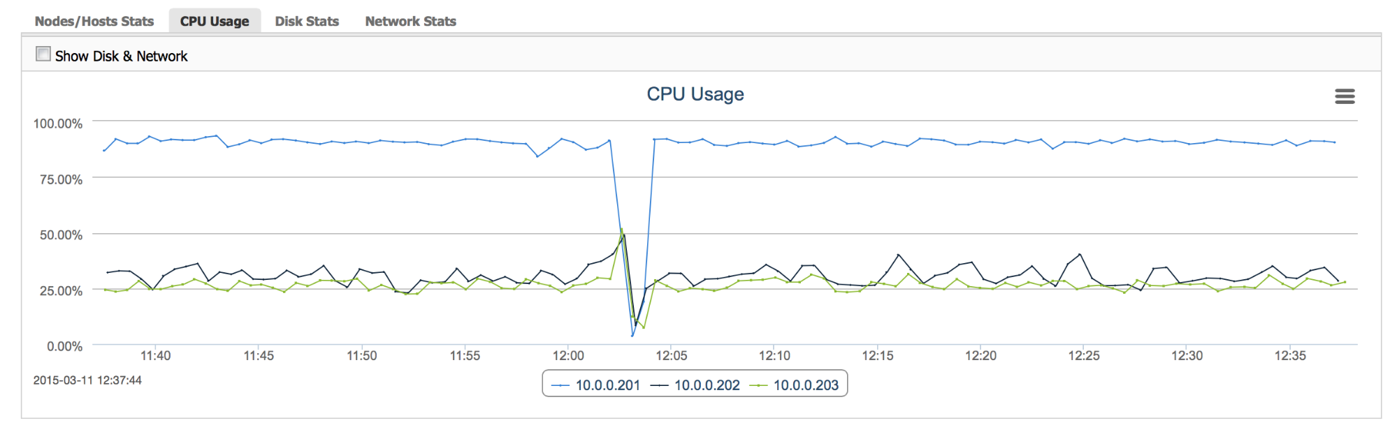
“CPU Usage” – this graph gives us a view of CPU utilization across all nodes – it’s easy to check the pattern – is the load stable or are there temporary spikes? Are all nodes loaded evenly or are some of them suffering more than others?
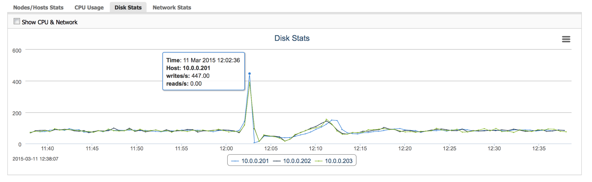
“Disk Stats” – this graph gives us information about disk utilization. It is not exactly the same data as we discussed previously, as here we are graphing I/O operations, not throughput. This graph should be used along with I/O throughput information as IOPS and MB/s which, while somehow related, they have their own respective bottlenecks. For example, bursts of random access (for example caused by an index scan in MySQL) may not cause high throughput measured in megabytes per second but I/O operations per second may skyrocket and hit the limitations of the underlying storage.
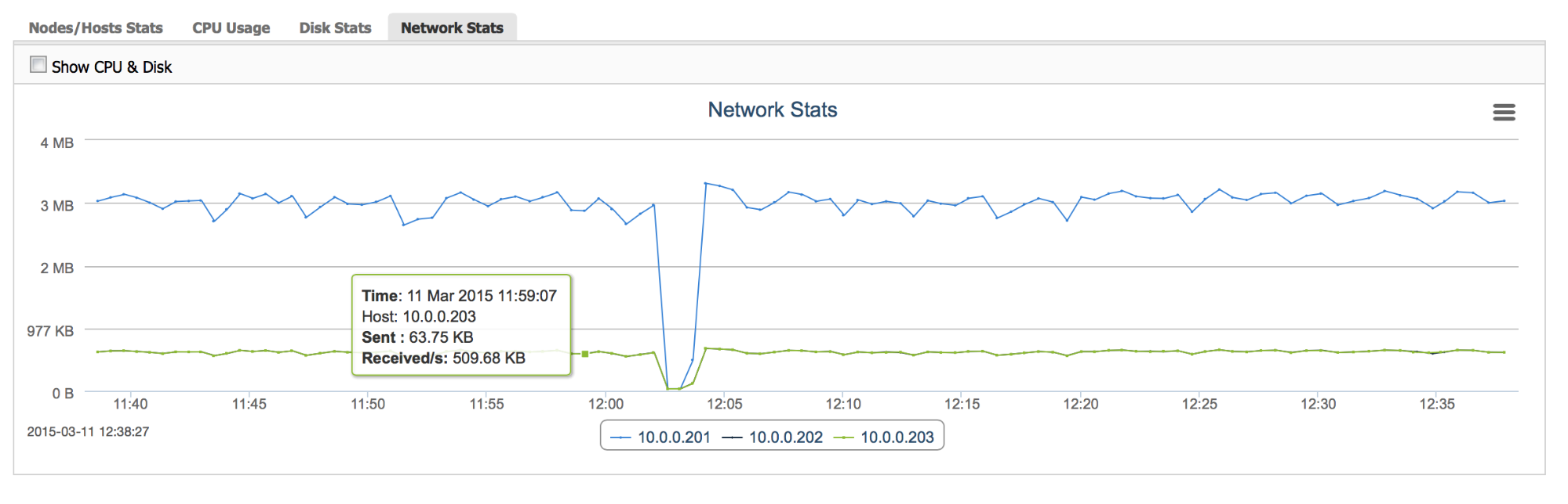
“Network Stats” gives an insight into how the network load changed with time – it is useful to see patterns in the workload and to be able to react before you hit the hardware’s limitation.
To close the subject of node’s health monitoring, let’s take a look into “Nodes” tab and pick one of the cluster nodes:
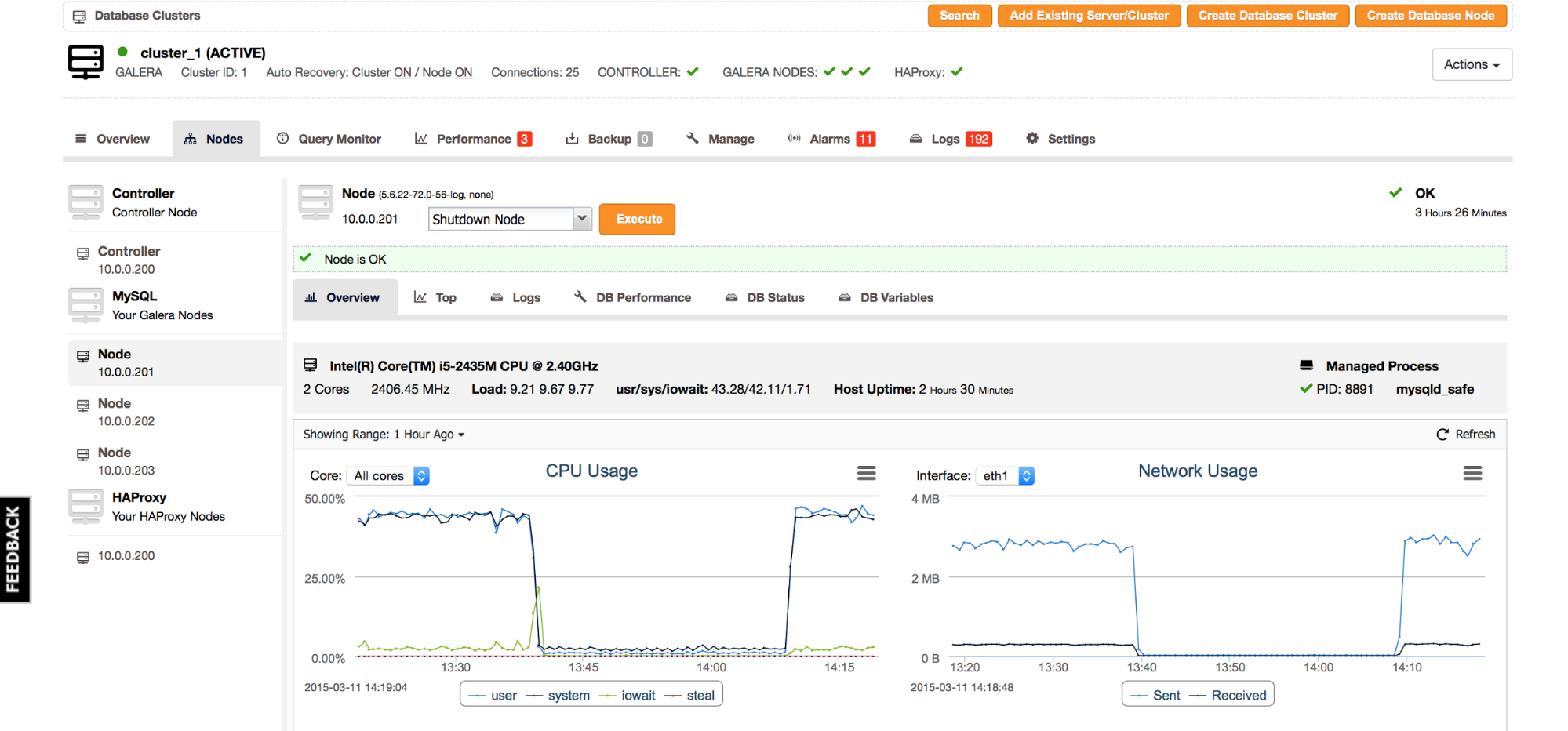
As we can see, there is some information on the node’s hardware – which CPU it is and how many cores are available. We can also get information about which processes are managed on it (MySQL in this case) and it’s pid. Uptime and Load data is the same information that we reviewed earlier but there is one more interesting bit. Previously we could check the CPU utilization, here we have information about how the different types of CPU utilization. “Usr” – this is CPU spent in userspace, in this node it’s most likely MySQL itself. “Sys” – system CPU utilization – time spent in the kernel. It could be caused by various types of workload. For example, it can be caused by a large number of interrupts caused by network or I/O utilization, it can also be caused by context switching inside of MySQL (mutex contention resulting in os_waits). Last part – “iowait” tells us how often processes had to wait for an I/O request.
By looking at the screenshot above, we can tell that load is high and user/system CPU utilization is close to a 1:1 ratio. It means that something is not entirely correct with this node and we may have to dig deeper.
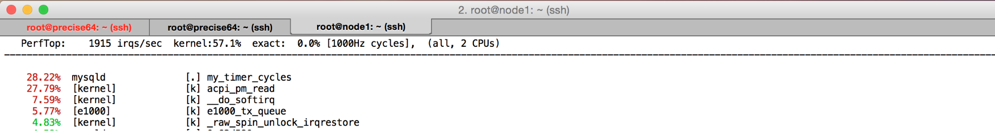
So, we used a CLI tool called perf to investigate what’s causing such a heavy system load. One of the calls (acpi_pm_read) has some links to the virtualization method used (VirtualBox) and we managed to modify the VM’s config to get more performance. And it all started from a quick look at the CPU utilization distribution data. Obviously, in production, this could give real gains in terms of faster applications and happier customers.
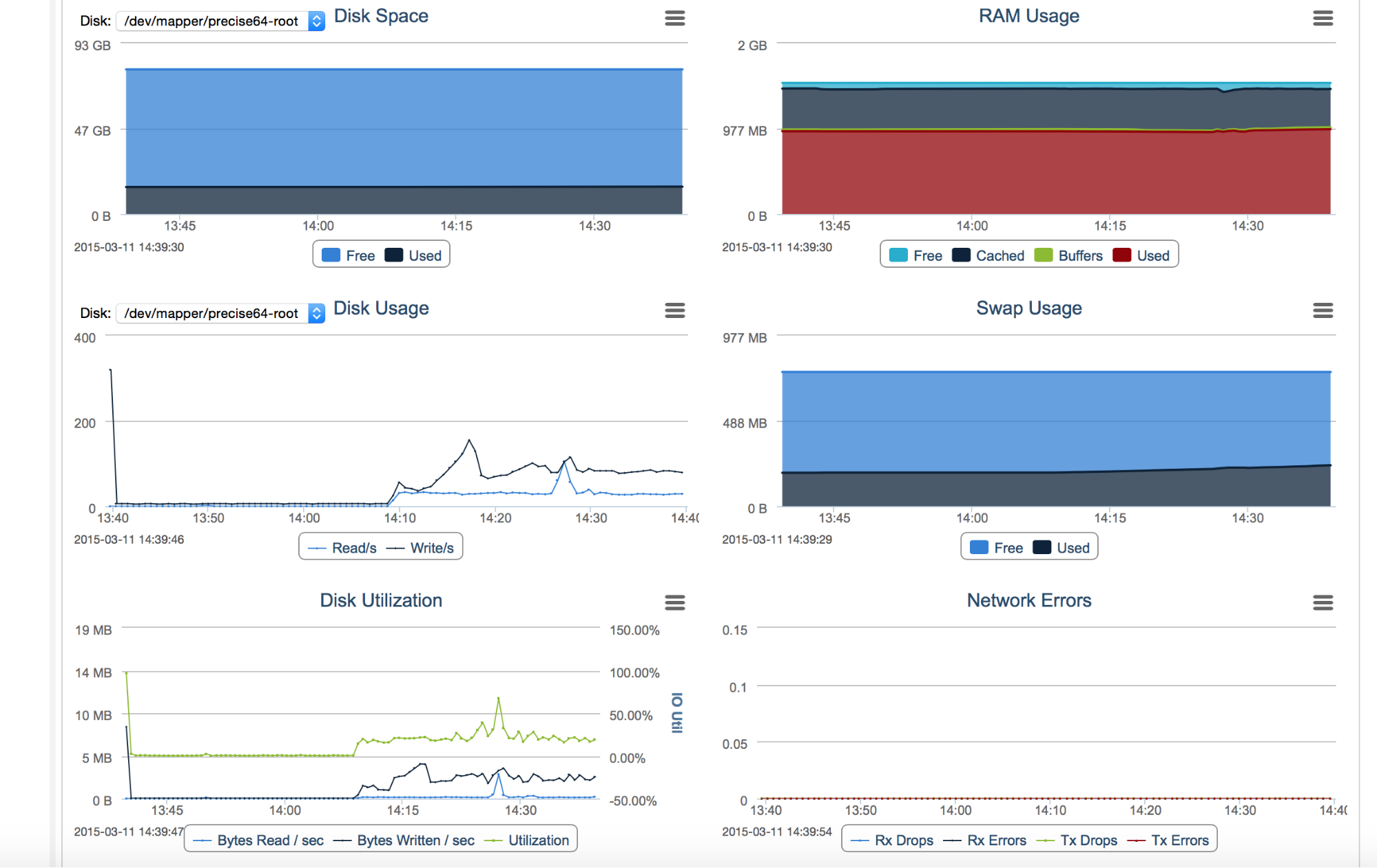
Most of graphs that you see in “Nodes” tab are similar to ones we discussed above. What’s new is a “Disk Utilization” graph, which shows us how disk throughput changed in time, “Disk Space”, which tells us how much free disk we have, “Network Errors”, which is self-explanatory and memory-related graphs.
“RAM Usage” tells us how the memory utilization looks like. If MySQL is the only large process on the node and if all of the tables use the InnoDB engine, what we’ll see is most often large chunks, even up to 80%, of memory used for MySQL’s InnoDB buffer pool. The rest of the memory will be most likely used by the Linux cache. Memory represented by “Cache” and “Buffers” is used by the OS to cache files (there’s a distinction between those two but it’s mostly irrelevant) – for the MySQL node, this would be mostly log files: relay logs, binary logs, InnoDB redo logs (depending on the MySQL’s configuration) and other data, frequently used by the operating system.
“Swap Usage” gives us information about swapfile utilization. If Linux needs to free some memory for a new process, it may use swap file to store old content. Ideally, we don’t want a node to swap but for that I mean swap actively. It’s not a problem when the OS writes something to a swap file and then forgets about it. More impacting are constant reads/writes, which tells us that there’s simply not enough memory for all processes and we need to tune down MySQL’s buffers.
At the time of writing, there’s no way of checking the swap activity from the ClusterControl UI, but if we see that swap is increasing, we should probably check it from CLI. One of useful commands is vmstat:
root@node1:~# vmstat 1 10
procs -----------memory---------- ---swap-- -----io---- -system-- ----cpu----
 r  b   swpd   free   buff  cache   si   so    bi    bo   in   cs us sy id wa
 9  0  27448  65264  22020 417452    0    6   189  1085 1972 1314 49 40  8  3
12  0  27752  75744  20396 408800    0  304   264  2524 3158 1552 41 51  7  1
 9  0  27752  75804  20436 409108    0    0   168  1892 3997 2598 52 45  3  1
 2  0  27752  75048  20476 409380    0    0   316  1964 3213 2275 47 45  5  3
14  1  27752  74504  20500 409612    0    0    88  1720 2588 1839 46 49  4  1
13  0  27752  73988  20524 410156    0    0   368  1288 3521 2185 48 49  2  1
10  0  27752  73880  20580 410464    0    0   100  2388 4058 2664 52 43  3  2
17  0  27752  73532  20612 410704    0    0    88  1860 3230 2200 50 43  6  1
12  0  27752  73716  20652 410972    0    0    72  1444 3175 2034 51 46  1  1
12  0  27752  72980  20692 411280    0    0   124  1952 3977 2602 55 39  5  2
We are interested in “si” – swap in and “so” – swap out columns. Naming convention is slightly counterintuitive as it’s from the kernel perspective so “swap in” means – read data from swap into kernel and “swap out” means write data out of kernel into a swap.
As we can see, there’s not much going on in this 10 seconds sample that I run – some data was written to swap but nothing was read. It means this node is probably not really impacted by the swapping.
This was a quick dive into some basic operating system metrics – there’s much more into it than what we covered here. Hopefully the information from this blog post will come handy some day, even if only to point you in the right direction. Have anything to add? We’d love to hear your thoughts!