blog
Database Indexing in PostgreSQL

Database Indexing is the use of special data structures that aim at improving performance, by achieving direct access to data pages. A database index works like the index section of a printed book: by looking in the index section, it is much faster to identify the page(s) which contain the term we are interested in. We can easily locate the pages and access them directly. This is instead of scanning the pages of the book sequentially, till we find the term we are looking for.
Indexes are an essential tool in the hands of a DBA. Using indexes can provide great performance gains for a variety of data domains. PostgreSQL is known for its great extensibility and the rich collection of both core and 3rd party addons, and indexing is no exception to this rule. PostgreSQL indexes cover a rich spectrum of cases, from the simplest b-tree indexes on scalar types to geospatial GiST indexes to fts or json or array GIN indexes.
Indexes, however, as wonderful as they seem (and actually are!) don’t come for free. There is a certain penalty that goes with writes on an indexed table. So the DBA, before examining her options to create a specific index, should first make sure that the said index makes sense in the first place, meaning that the gains from its creation will outweigh the performance loss on writes.
PostgreSQL Basic Index Terminology
Before describing the types of indexes in PostgreSQL and their use, let’s take a look at some terminology that any DBA will come across sooner or later when reading the docs.
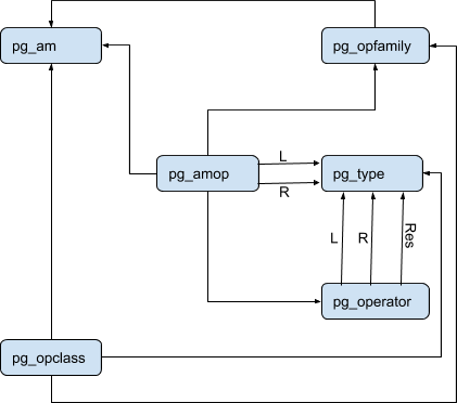
- Index Access Method (also called as Access Method): The index type (B-tree, GiST, GIN, etc)
- Type: the data type of the indexed column
- Operator: a function between two data types
- Operator Family: cross data type operator, by grouping operators of types with similar behaviour
- Operator Class (also mentioned as index strategy): defines the operators to be used by the index for a column
In PostgreSQL’s system catalog, access methods are stored in pg_am, operator classes in pg_opclass, operator families in pg_opfamily. The dependencies of the above are shown in the diagram below:
Types of Indexes in PostgreSQL
PostgreSQL provides the following Index types:
- B-tree: the default index, applicable for types that can be sorted
- Hash: handles equality only
- GiST: suitable for non-scalar data types (e.g. geometrical shapes, fts, arrays)
- SP-GiST: space partitioned GIST, an evolution of GiST for handling non-balanced structures (quadtrees, k-d trees, radix trees)
- GIN: suitable for complex types (e.g. jsonb, fts, arrays )
- BRIN: a relatively new type of index which supports data that can be sorted by storing min/max values in each block
Low we’ll try to get our hands dirty with some real world examples. All examples given are done with PostgreSQL 10.0 (with both 10 and 9 psql clients) on FreeBSD 11.1.
B-tree Indexes
Let’s suppose we have the following table:
create table part (
id serial primary key,
partno varchar(20) NOT NULL UNIQUE,
partname varchar(80) NOT NULL,
partdescr text,
machine_id int NOT NULL
);
testdb=# d part
                                  Table "public.part"
   Column       |         Type          |                     Modifiers
------------+-----------------------+---------------------------------------------------
 id         | integer                 | not null default nextval('part_id_seq'::regclass)
 partno     | character varying(20)| not null
 partname       | character varying(80)| not null
 partdescr      | text                    |
 machine_id     | integer                 | not null
Indexes:
    "part_pkey" PRIMARY KEY, btree (id)
    "part_partno_key" UNIQUE CONSTRAINT, btree (partno)
When we define this rather common table, PostgreSQL creates two unique B-tree indexes behind the scenes: part_pkey and part_partno_key. So every unique constraint in PostgreSQL is implemented with a unique INDEX. Lets populate our table with a million rows of data:
testdb=# with populate_qry as (select gs from generate_series(1,1000000) as gs )
insert into part (partno, partname,machine_id) SELECT 'PNo:'||gs, 'Part '||gs,0 from populate_qry;
INSERT 0 1000000
Now let’s try to do some queries on our table. First we tell psql client to report query times by typing timing:
testdb=# select * from part where id=100000;
   id   |   partno   |  partname   | partdescr | machine_id
--------+------------+-------------+-----------+------------
 100000 | PNo:100000 | Part 100000 |           |          0
(1 row)

Time: 0,284 ms
testdb=# select * from part where partno='PNo:100000';
id | partno | partname | partdescr | machine_id
--------+------------+-------------+-----------+------------
100000 | PNo:100000 | Part 100000 | | 0
(1 row)
Time: 0,319 msWe observe that it takes only fractions of the millisecond to get our results. We expected this since for both columns used in the above queries, we have already defined the appropriate indexes. Now let’s try to query on column partname, for which no index exists.
testdb=# select * from part where partname='Part 100000';
   id   |   partno   |  partname   | partdescr | machine_id
--------+------------+-------------+-----------+------------
 100000 | PNo:100000 | Part 100000 |           |          0
(1 row)

Time: 89,173 ms
Here we see clearly that for the non indexed column, the performance drops significantly. Now lets create an index on that column, and repeat the query:
testdb=# create index part_partname_idx ON part(partname);
CREATE INDEX
Time: 15734,829 ms (00:15,735)
testdb=# select * from part where partname='Part 100000';
   id   |   partno   |  partname   | partdescr | machine_id
--------+------------+-------------+-----------+------------
 100000 | PNo:100000 | Part 100000 |           |          0
(1 row)

Time: 0,525 ms
Our new index part_partname_idx is also a B-tree index (the default). First we note that the index creation on the million rows table took a significant amount of time, about 16 seconds. Then we observe that our query speed was boosted from 89 ms down to 0.525 ms. B-tree indexes, besides checking for equality, can also help with queries involving other operators on ordered types, such as <,<=,>=,>. Lets try with <= and >=
testdb=# select count(*) from part where partname>='Part 9999900';
 count
-------
     9
(1 row)

Time: 0,359 ms
testdb=# select count(*) from part where partname<='Part 9999900';
count
--------
999991
(1 row)
Time: 355,618 msThe first query is much faster than the second, by using the EXPLAIN (or EXPLAIN ANALYZE) keywords we can see if the actual index is used or not:
testdb=# explain select count(*) from part where partname>='Part 9999900';
                                       QUERY PLAN
-----------------------------------------------------------------------------------------
 Aggregate  (cost=8.45..8.46 rows=1 width=8)
   ->  Index Only Scan using part_partname_idx on part  (cost=0.42..8.44 rows=1 width=0)
         Index Cond: (partname >= 'Part 9999900'::text)
(3 rows)

Time: 0,671 ms
testdb=# explain select count(*) from part where partname<='Part 9999900';
QUERY PLAN
----------------------------------------------------------------------------------------
Finalize Aggregate (cost=14603.22..14603.23 rows=1 width=8)
-> Gather (cost=14603.00..14603.21 rows=2 width=8)
Workers Planned: 2
-> Partial Aggregate (cost=13603.00..13603.01 rows=1 width=8)
-> Parallel Seq Scan on part (cost=0.00..12561.33 rows=416667 width=0)
Filter: ((partname)::text <= 'Part 9999900'::text)
(6 rows)
Time: 0,461 msIn the first case, the query planner chooses to use the part_partname_idx index. We also observe that this will result in an index-only scan which means no access to the data tables at all. In the second case the planner determines that there is no point in using the index as the returned results are a big portion of the table, in which case a sequential scan is thought to be faster.
Hash Indexes
Use of hash indexes up to and including PgSQL 9.6 was discouraged due to reasons having to do with lack of WAL writing. As of PgSQL 10.0 those issues were fixed, but still hash indexes made little sense to use. There are efforts in PgSQL 11 to make hash indexes a first class index method along with its bigger brothers (B-tree, GiST, GIN). So, with this in mind, let’s actually try a hash index in action.
We will enrich our part table with a new column parttype and populate it with values of equal distribution, and then run a query that tests for parttype equal to ‘Steering’:
testdb=# alter table part add parttype varchar(100) CHECK (parttype in ('Engine','Suspension','Driveline','Brakes','Steering','General')) NOT NULL DEFAULT 'General';
ALTER TABLE
Time: 42690,557 ms (00:42,691)
testdb=# with catqry as  (select id,(random()*6)::int % 6 as cat from part)
update part SET parttype = CASE WHEN cat=1 THEN 'Engine' WHEN cat=2 THEN 'Suspension' WHEN cat=3 THEN 'Driveline' WHEN cat=4 THEN 'Brakes' WHEN cat=5 THEN 'Steering' ELSE 'General' END FROM catqry WHERE part.id=catqry.id;
UPDATE 1000000
Time: 46345,386 ms (00:46,345)
testdb=# select count(*) from part where id % 500 = 0 AND parttype = 'Steering';
 count
-------
   322
(1 row)

Time: 93,361 ms
Now we create a Hash index for this new column, and retry the previous query:
testdb=# create index part_parttype_idx ON part USING hash(parttype);
CREATE INDEX
Time: 95525,395 ms (01:35,525)
testdb=# analyze ;
ANALYZE
Time: 1986,642 ms (00:01,987)
testdb=# select count(*) from part where id % 500 = 0 AND parttype = 'Steering';
 count
-------
   322
(1 row)

Time: 63,634 ms
We note the improvement after using the hash index. Now we will compare the performance of a hash index on integers against the equivalent b-tree index.
testdb=# update part set machine_id = id;
UPDATE 1000000
Time: 392548,917 ms (06:32,549)
testdb=# select * from part where id=500000;
   id   |   partno   |  partname   | partdescr | machine_id |  parttype
--------+------------+-------------+-----------+------------+------------
 500000 | PNo:500000 | Part 500000 |           |     500000 | Suspension
(1 row)

Time: 0,316 ms
testdb=# select * from part where machine_id=500000;
id | partno | partname | partdescr | machine_id | parttype
--------+------------+-------------+-----------+------------+------------
500000 | PNo:500000 | Part 500000 | | 500000 | Suspension
(1 row)
Time: 97,037 mstestdb=# create index part_machine_id_idx ON part USING hash(machine_id);
CREATE INDEX
Time: 4756,249 ms (00:04,756)
testdb=#
testdb=# select * from part where machine_id=500000;
id | partno | partname | partdescr | machine_id | parttype
--------+------------+-------------+-----------+------------+------------
500000 | PNo:500000 | Part 500000 | | 500000 | Suspension
(1 row)
Time: 0,297 msAs we see, with the use of hash indexes, the speed of queries that check for equality is very close to the speed of B-tree indexes. Hash indexes are said to be marginally faster for equality than B-trees, in fact we had to try each query two or three times until hash index gave a better result than the b-tree equivalent.
GiST Indexes
GiST (Generalized Search Tree) is more than a single kind of index, but rather an infrastructure to build many indexing strategies. The default PostgreSQL distribution provides support for geometric data types, tsquery and tsvector. In contrib there are implementations of many other operator classes. By reading the docs and the contrib dir, the reader will observe that there is a rather big overlap between GiST and GIN use cases: int arrays, full text search to name the main cases. In those cases GIN is faster, and the official documentation explicitly states that. However, GiST provides extensive geometric data type support. Also, as at the time of this writing, GiST (and SP-GiST) is the only meaningful method that can be used with exclusion constraints. We will see an example on this. Let us suppose (staying in the field of mechanical engineering) that we have a requirement to define machines type variations for a particular machine type, that are valid for a certain period in time; and that for a particular variation, no other variation can exist for the same machine type whose period in time overlaps (conflicts) with the particular variation period.
create table machine_type (
	id SERIAL PRIMARY KEY,
	mtname varchar(50) not null,
	mtvar varchar(20) not null,
	start_date date not null,
	end_date date,
	CONSTRAINT machine_type_uk UNIQUE (mtname,mtvar)
);
Above we tell PostgreSQL that for every machine type name (mtname) there can be only one variation (mtvar). Start_date denotes the starting date of the period in which this machine type variation is valid, and end_date denotes the ending date of this period. Null end_date means that the machine type variation is currently valid. Now we want to express the non-overlapping requirement with a constraint. The way to do this is with an exclusion constraint:
testdb=# alter table machine_type ADD CONSTRAINT machine_type_per EXCLUDE USING GIST (mtname WITH =,daterange(start_date,end_date) WITH &&);The EXCLUDE PostgreSQL syntax allows us to specify many columns of different types and with a different operator for each one. && is the overlapping operator for date ranges, and = is the common equality operator for varchar. But as long as we hit enter PostgreSQL complains with a message:
ERROR:  data type character varying has no default operator class for access method "gist"
HINT:  You must specify an operator class for the index or define a default operator class for the data type.
What is lacking here is GiST opclass support for varchar. Provided we have successfully built and installed the btree_gist extension, we may proceed with creating the extension:
testdb=# create extension btree_gist ;
CREATE EXTENSION
And then re-trying to create the constraint and test it:
testdb=# alter table machine_type ADD CONSTRAINT machine_type_per EXCLUDE USING GIST (mtname WITH =,daterange(start_date,end_date) WITH &&);
ALTER TABLE
testdb=# insert into machine_type (mtname,mtvar,start_date,end_date) VALUES('Subaru EJ20','SH','2008-01-01','2013-01-01');
INSERT 0 1
testdb=# insert into machine_type (mtname,mtvar,start_date,end_date) VALUES('Subaru EJ20','SG','2002-01-01','2009-01-01');
ERROR:  conflicting key value violates exclusion constraint "machine_type_per"
DETAIL:  Key (mtname, daterange(start_date, end_date))=(Subaru EJ20, [2002-01-01,2009-01-01)) conflicts with existing key (mtname, daterange(start_date, end_date))=(Subaru EJ20, [2008-01-01,2013-01-01)).
testdb=# insert into machine_type (mtname,mtvar,start_date,end_date) VALUES('Subaru EJ20','SG','2002-01-01','2008-01-01');
INSERT 0 1
testdb=# insert into machine_type (mtname,mtvar,start_date,end_date) VALUES('Subaru EJ20','SJ','2013-01-01',null);
INSERT 0 1
testdb=# insert into machine_type (mtname,mtvar,start_date,end_date) VALUES('Subaru EJ20','SJ2','2018-01-01',null);
ERROR:  conflicting key value violates exclusion constraint "machine_type_per"
DETAIL:  Key (mtname, daterange(start_date, end_date))=(Subaru EJ20, [2018-01-01,)) conflicts with existing key (mtname, daterange(start_date, end_date))=(Subaru EJ20, [2013-01-01,)).
SP-GiST Indexes
SP-GiST which stands for space-partitioned GiST, like GiST, is an infrastructure that enables the development for many different strategies in the domain of non-balanced disk-based data structures. The default PgSQL distribution offers support for two-dimensional points, (any type) ranges, text and inet types. Like GiST, SP-GiST can be used in exclusion constraints, in a similar way to the example shown in the previous chapter.
GIN Indexes
GIN (Generalized Inverted Index) like GiST and SP-GiST can provide many indexing strategies. GIN is suited when we want to index columns of composite types. The default PostgreSQL distribution provides support for any array type, jsonb and full text search (tsvector). In contrib there are implementations of many other operator classes. Jsonb, a highly praised feature of PostgreSQL (and a relatively recent (9.4+) development) is relying on GIN for index support. Another common use of GIN is indexing for full text search. Full text search in PgSQL deserves an article on its own, so we’ll cover here only the indexing part. First let’s make some preparation to our table, by giving not null values to partdescr column and updating a single row with a meaningful value:
testdb=# update part set partdescr ='';
UPDATE 1000000
Time: 383407,114 ms (06:23,407)
testdb=# update part set partdescr = 'thermostat for the cooling system' where id=500000;
UPDATE 1
Time: 2,405 ms
Then we perform a text search on the newly updated column:
testdb=# select * from part where partdescr @@ 'thermostat';
   id   |   partno   |  partname   |             partdescr             | machine_id |  parttype
--------+------------+-------------+-----------------------------------+------------+------------
 500000 | PNo:500000 | Part 500000 | thermostat for the cooling system |     500000 | Suspension
(1 row)

Time: 2015,690 ms (00:02,016)
This is quite slow, almost 2 seconds to bring our result. Now let’s try to create a GIN index on type tsvector, and repeat the query, using an index-friendly syntax:
testdb=# CREATE INDEX part_partdescr_idx ON part USING gin(to_tsvector('english',partdescr));
CREATE INDEX
Time: 1431,550 ms (00:01,432)
testdb=# select * from part where to_tsvector('english',partdescr) @@ to_tsquery('thermostat');
   id   |   partno   |  partname   |             partdescr             | machine_id |  parttype
--------+------------+-------------+-----------------------------------+------------+------------
 500000 | PNo:500000 | Part 500000 | thermostat for the cooling system |     500000 | Suspension
(1 row)

Time: 0,952 ms
And we get a 2000-fold speed up. Also we may note the relatively short time that it took the index to be created. You may experiment with using GiST instead of GIN in the above example, and measure the performance of reads, writes and index creation for both access methods.
BRIN Indexes
BRIN (Block Range Index) is the newest addition to the PostgreSQL’s set of index types, since it was introduced in PostgreSQL 9.5, having only a few years as a standard core feature. BRIN works on very large tables by storing summary information for a set of pages called “Block Range”. BRIN Indexes are lossy (like GiST) and this requires both extra logic in PostgreSQL’s query executor, and also the need for extra maintenance. Let’s see BRIN in action:
testdb=# select count(*) from part where machine_id BETWEEN 5000 AND 10000;
 count
-------
  5001
(1 row)

Time: 100,376 ms
testdb=# create index part_machine_id_idx_brin ON part USING BRIN(machine_id);
CREATE INDEX
Time: 569,318 ms
testdb=# select count(*) from part where machine_id BETWEEN 5000 AND 10000;
count
-------
5001
(1 row)
Time: 5,461 msHere we see on average a ~ 18-fold speedup by the use of the BRIN index. However, BRIN’s real home is in the domain of big data, so we hope to test this relatively new technology in real world scenarios in the future.